Two-Way ANOVA in R: Two Factors and Their Interaction

Test two grouping factors at once — their main effects and the interaction between them — rstatix the modern way, base R for the classic table

Learn to run a two-way ANOVA in R to test the effect of two factors and their interaction on a numeric outcome. Use rstatix anova_test() for a tidy table with a ges effect size, and base R aov() + summary() for the classic layout — with the equal-variance and normality assumption checks, how to read the two main effects and the interaction term, what a significant interaction means, simple-main-effect post-hoc comparisons, and a boxplot with the p-values on it.

TipKey takeaways

• A two-way ANOVA tests two grouping factors at once — each factor’s main effect plus the interaction between them — on a single numeric outcome.
• Use anova_test() from rstatix with a outcome ~ A * B formula for a tidy table (F, p, and the ges effect size for each term), or base R aov() + summary() for the classic layout.
• The interaction term (A:B) is the point of a two-way ANOVA: a significant interaction means the effect of one factor depends on the level of the other — interpret it before the main effects.
• Check the same two assumptions: homogeneity of variance (levene_test() on the cells) and normality of residuals (shapiro_test() on the model residuals).
• When the interaction is significant, follow up with simple main effects — split the data by one factor and run a one-way analysis inside each level — then plot the result with the p-values on it (stat_pvalue_manual()).

Introduction

A two-way ANOVA (analysis of variance) answers a richer question than the one-way version: how do two factors — and their combination — affect the outcome? Instead of one grouping variable, the data are cross-classified by two factors (call them A and B), and the test splits the variation in the outcome into a main effect of A, a main effect of B, and an interaction A:B.

The interaction is the real reason to run a two-way ANOVA. An interaction occurs when the effect of one factor changes depending on the level of the other — for example, when education raises job satisfaction more for one gender than the other. This lesson runs the whole workflow two ways — the modern, pipe-friendly rstatix anova_test() and the classic base-R aov() — using the jobsatisfaction dataset, and shows the assumption checks, the simple-main-effect follow-ups, and how to put the p-values on the plot.

Note

Two-way ANOVA hypotheses. Three null hypotheses: (1) factor A’s group means are equal, (2) factor B’s group means are equal, and (3) there is no interaction between A and B (the effect of A is the same at every level of B). A significant interaction means hypothesis 3 is rejected — the factors do not act independently.

The data: two factors at once

We use the jobsatisfaction dataset from the datarium package — job satisfaction score for 58 people, organized by gender (male, female) and education_level (school, college, university). The research question: is there a significant interaction between gender and education level on job satisfaction? Here education_level is the focal variable (our primary concern) and gender is the moderator — we ask whether education’s effect depends on gender.

library(rstatix)

set.seed(123)
data("jobsatisfaction", package = "datarium")

# one random row per gender × education_level cell
jobsatisfaction %>% sample_n_by(gender, education_level, size = 1)

# A tibble: 6 × 4
  id    gender education_level score
  <fct> <fct>  <fct>           <dbl>
1 3     male   school           5.07
2 12    male   college          6.45
3 28    male   university       8.7 
4 30    female school           5.94
5 44    female college          7.1 
6 53    female university       9.42

gender (2 levels) and education_level (3 levels) make a 2 × 3 factorial design, and the outcome is score. Summarize each cell with get_summary_stats() — the count, mean and standard deviation per combination, the numbers behind the plots that follow:

library(rstatix)

data("jobsatisfaction", package = "datarium")

jobsatisfaction %>%
  group_by(gender, education_level) %>%
  get_summary_stats(score, type = "mean_sd")

# A tibble: 6 × 6
  gender education_level variable     n  mean    sd
  <fct>  <fct>           <fct>    <dbl> <dbl> <dbl>
1 male   school          score        9  5.43 0.364
2 male   college         score        9  6.22 0.34 
3 male   university      score       10  9.29 0.445
4 female school          score       10  5.74 0.474
5 female college         score       10  6.46 0.475
6 female university      score       10  8.41 0.938

Look at the data first

Always plot before testing. A boxplot of score by gender, coloured by education_level, shows the six cells side by side:

library(ggpubr)

data("jobsatisfaction", package = "datarium")

ggboxplot(
  jobsatisfaction, x = "gender", y = "score",
  color = "education_level", palette = "jco",
  xlab = "Gender", ylab = "Job satisfaction score"
)

An interaction plot (ggline() with add = "mean_se", coloured by the second factor) is the most telling view of an interaction: it draws each cell’s mean, and non-parallel lines suggest an interaction — the education gap is not identical across genders:

library(ggpubr)

data("jobsatisfaction", package = "datarium")

ggline(
  jobsatisfaction, x = "gender", y = "score", color = "education_level",
  add = "mean_se", palette = "jco",
  xlab = "Gender", ylab = "Job satisfaction score"
)

Run the two-way ANOVA

With rstatix (recommended)

anova_test() takes the data and an outcome ~ A * B formula. The * asks for both main effects and the interaction (gender * education_level expands to gender + education_level + gender:education_level). The result is a tidy table — one row per term:

library(rstatix)

data("jobsatisfaction", package = "datarium")

res.aov <- jobsatisfaction %>% anova_test(score ~ gender * education_level)
res.aov

ANOVA Table (type II tests)

                  Effect DFn DFd       F        p p<.05   ges
1                 gender   1  52   0.745 3.92e-01       0.014
2        education_level   2  52 187.892 1.60e-24     * 0.878
3 gender:education_level   2  52   7.338 2.00e-03     * 0.220

Read it row by row: gender (main effect), education_level (main effect), and gender:education_level (the interaction). Each row gives F, DFn/DFd, p, a p<.05 flag, and ges — the generalized eta-squared effect size. There is a statistically significant interaction between gender and education level, F(2, 52) = 7.34, p = 0.002 — so the effect of education on satisfaction depends on gender.

Tip

* vs : in the formula. gender * education_level fits both main effects and the interaction. gender:education_level alone is the interaction term only. Use the A * B form for a standard two-way ANOVA; switch to the additive model score ~ gender + education_level (no interaction) only when the interaction is not significant.

Tip

Run it on your own data. Load your file — mydata <- read.csv("my-file.csv") — make both grouping columns factors (mydata$A <- factor(mydata$A)), then pipe it in: mydata %>% anova_test(outcome ~ A * B).

With base R

aov() fits the model and summary() prints the classic ANOVA table — one line per term:

data("jobsatisfaction", package = "datarium")

res.aov.base <- aov(score ~ gender * education_level, data = jobsatisfaction)
summary(res.aov.base)

                       Df Sum Sq Mean Sq F value  Pr(>F)    
gender                  1   0.54    0.54   1.787 0.18709    
education_level         2 113.68   56.84 187.892 < 2e-16 ***
gender:education_level  2   4.44    2.22   7.338 0.00156 ** 
Residuals              52  15.73    0.30                    
---
Signif. codes:  0 '***' 0.001 '**' 0.01 '*' 0.05 '.' 0.1 ' ' 1

The rows are gender, education_level, gender:education_level and the Residuals; F value and Pr(>F) (with significance stars) carry the same conclusion as the rstatix call. aov() simply prints the textbook layout and keeps the fitted model for the diagnostics and post-hoc tests below.

Warning

Why the gender p-value differs between the two tables. jobsatisfaction is slightly unbalanced (9–10 observations per cell), and on an unbalanced design the two engines use different sums of squares: base summary(aov()) uses Type-I (sequential, order-dependent), while anova_test() defaults to Type-II. So the gender main effect reads p = 0.19 (base) vs p = 0.39 (rstatix) — both non-significant, same conclusion, different number. The interaction term is identical either way. For a base-R table that matches rstatix exactly, use a Type-II test: car::Anova(res.aov.base, type = 2).

NoteThe math (optional)

A two-way ANOVA partitions the total variation in the outcome into the parts each term explains plus what’s left over — the total (T), the two main effects (A, B), their interaction (AB) and the residual (R):

\[SS_T = SS_A + SS_B + SS_{AB} + SS_R\]

Each sum of squares becomes a mean square by dividing by its degrees of freedom, \(MS = SS / df\), and each term’s F-statistic is its mean square over the residual mean square:

\[F_A = \frac{MS_A}{MS_R}, \quad F_B = \frac{MS_B}{MS_R}, \quad F_{AB} = \frac{MS_{AB}}{MS_R}\]

So there is one F per term — \(F_A\), \(F_B\) and the interaction \(F_{AB}\) — each comparing the variation that term explains against the unexplained (within-cell) variation. A large F means the term accounts for more variation than chance alone would, which is what the p-value formalizes.

Effect size: how big is each term?

A significant p-value says a term matters; the effect size says how much. anova_test() already prints ges (generalized eta-squared) per term. For the classic eta-squared, eta_squared() works on the fitted aov() model:

library(rstatix)

data("jobsatisfaction", package = "datarium")

eta_squared(aov(score ~ gender * education_level, data = jobsatisfaction))

                gender        education_level gender:education_level 
           0.004022942            0.845889912            0.033035192 

education_level explains by far the largest share of the variation, gender very little, and the gender:education_level interaction a small but real share — report the effect size alongside each p-value, not just “p < 0.05”. As a rough benchmark, η² ≈ 0.01 is small, ≈ 0.06 medium and ≥ 0.14 large: education_level’s ges ≈ 0.88 is very large, gender’s ≈ 0.01 is small, and the interaction’s 0.22 is large.

Check the assumptions

A two-way ANOVA trusts the same assumptions as the one-way test (beyond independent observations): no extreme outliers, the residuals are normally distributed, and the cells have equal variance.

Outliers

identify_outliers() flags extreme values in each cell — an empty result means none would distort the cell means:

library(rstatix)

data("jobsatisfaction", package = "datarium")

jobsatisfaction %>%
  group_by(gender, education_level) %>%
  identify_outliers(score)

[1] gender          education_level id              score          
[5] is.outlier      is.extreme     
<0 lignes> (ou 'row.names' de longueur nulle)

There were no extreme outliers.

Homogeneity of variance — Levene’s test

Levene’s test asks whether the six cells share a common variance. Cross both factors in the formula so it tests every cell; p > 0.05 means no evidence the variances differ — what we want:

library(rstatix)

data("jobsatisfaction", package = "datarium")

jobsatisfaction %>% levene_test(score ~ gender * education_level)

# A tibble: 1 × 4
    df1   df2 statistic      p
  <int> <int>     <dbl>  <dbl>
1     5    52      2.20 0.0686

A non-significant Levene’s test means equal-variance holds across the cells. Back it with the residuals-vs-fitted plot — an even band of points across the fitted cell means (no funnel shape) confirms constant variance:

data("jobsatisfaction", package = "datarium")
model <- aov(score ~ gender * education_level, data = jobsatisfaction)

plot(model, 1)   # residuals vs fitted — a flat band = equal variance

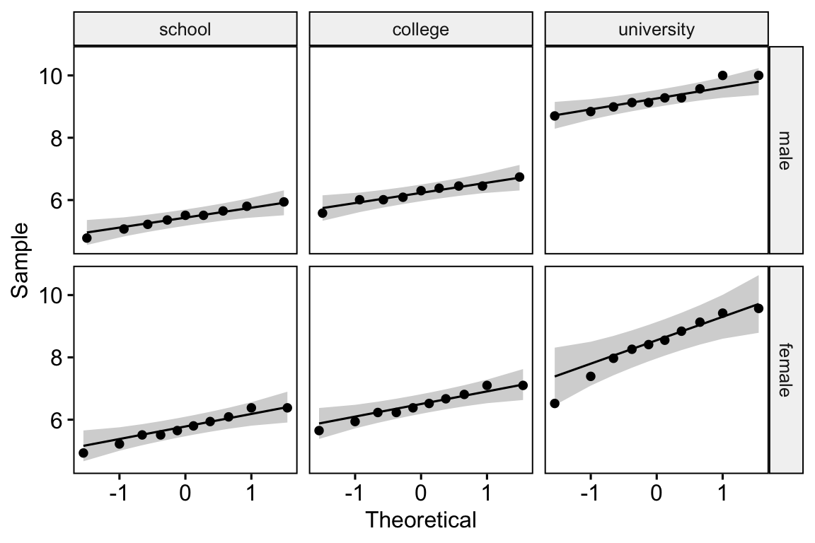
Normality of residuals — Shapiro-Wilk + Q-Q

ANOVA assumes the residuals (not each raw cell) are normal. Fit the model, test the residuals with Shapiro-Wilk (p > 0.05 → no departure from normal), and back it with a Q-Q plot:

library(rstatix)

data("jobsatisfaction", package = "datarium")

model <- lm(score ~ gender * education_level, data = jobsatisfaction)
shapiro_test(residuals(model))

# A tibble: 1 × 3
  variable         statistic p.value
  <chr>                <dbl>   <dbl>
1 residuals(model)     0.968   0.127

library(ggpubr)

data("jobsatisfaction", package = "datarium")
model <- lm(score ~ gender * education_level, data = jobsatisfaction)

ggqqplot(residuals(model))

With only a few groups you can also check normality within each cell — shapiro_test() grouped by both factors, and a Q-Q plot faceted by the cell:

library(rstatix)

data("jobsatisfaction", package = "datarium")

jobsatisfaction %>%
  group_by(gender, education_level) %>%
  shapiro_test(score)

# A tibble: 6 × 5
  gender education_level variable statistic     p
  <fct>  <fct>           <chr>        <dbl> <dbl>
1 male   school          score        0.980 0.966
2 male   college         score        0.958 0.779
3 male   university      score        0.916 0.323
4 female school          score        0.963 0.819
5 female college         score        0.963 0.819
6 female university      score        0.950 0.674

library(ggpubr)

data("jobsatisfaction", package = "datarium")

ggqqplot(jobsatisfaction, "score", facet.by = c("gender", "education_level"))

The score was normally distributed in each cell (p > 0.05).

Note

If the residuals stray far from the line, or Levene’s test is significant, the data don’t fit the classic two-way ANOVA. See the dedicated normality test lesson for the full assumption workflow and the non-parametric routes.

Interpreting a significant interaction

The interaction term is the heart of a two-way ANOVA, so interpret it first:

• No significant interaction → the factors act independently. Read the two main effects as in a one-way ANOVA, and consider re-fitting the simpler additive model score ~ gender + education_level.
• Significant interaction (our case) → the effect of one factor depends on the level of the other, so a single “main effect” can mislead. Don’t over-interpret the main effects in isolation — instead, break the interaction into simple main effects: the effect of one factor within each level of the other.

Post-hoc: simple main effects

When the interaction is significant, the right follow-up is simple main effects — analyse the focal variable within each level of the moderator. Here we ask: does education level matter within each gender? Group by gender, then run a one-way anova_test(), passing the overall model as error so it uses the pooled error term from the two-way model:

library(rstatix)

data("jobsatisfaction", package = "datarium")

model <- lm(score ~ gender * education_level, data = jobsatisfaction)
jobsatisfaction %>%
  group_by(gender) %>%
  anova_test(score ~ education_level, error = model)

# A tibble: 2 × 8
  gender Effect            DFn   DFd     F        p `p<.05`   ges
* <fct>  <chr>           <dbl> <dbl> <dbl>    <dbl> <chr>   <dbl>
1 male   education_level     2    52 132.  3.92e-21 *       0.836
2 female education_level     2    52  62.8 1.35e-14 *       0.707

The simple main effect of education level was statistically significant for both males (F(2, 52) = 132, p < 0.0001) and females (F(2, 52) = 62.8, p < 0.0001) — but the F-statistics differ, which is the interaction in action.

To see which education levels differ within each gender, follow with pairwise comparisons. emmeans_test() (estimated marginal means, a wrapper around the emmeans package) runs all pairwise comparisons with a Bonferroni adjustment:

library(rstatix)
library(emmeans)

data("jobsatisfaction", package = "datarium")

pwc <- jobsatisfaction %>%
  group_by(gender) %>%
  emmeans_test(score ~ education_level, p.adjust.method = "bonferroni")
pwc

# A tibble: 6 × 10
  gender term            .y.   group1  group2     df statistic        p    p.adj
* <fct>  <chr>           <chr> <chr>   <chr>   <dbl>     <dbl>    <dbl>    <dbl>
1 male   education_level score school  college    52     -3.07 3.37e- 3 1.01e- 2
2 male   education_level score school  univer…    52    -15.3  6.87e-21 2.06e-20
3 male   education_level score college univer…    52    -12.1  8.42e-17 2.53e-16
4 female education_level score school  college    52     -2.94 4.95e- 3 1.49e- 2
5 female education_level score school  univer…    52    -10.8  6.07e-15 1.82e-14
6 female education_level score college univer…    52     -7.90 1.84e-10 5.52e-10
# ℹ 1 more variable: p.adj.signif <chr>

Each row is one education-level pair within a gender: group1/group2 are the levels, and p.adj is the adjusted p-value. There was a significant difference in job satisfaction between all groups for both males and females (p < 0.05).

Plot it with the p-values on it

The publication-ready figure puts the test result on the plot — the overall ANOVA in the subtitle (get_test_label()) and the pairwise brackets via stat_pvalue_manual(), after add_xy_position() computes where the brackets sit:

library(rstatix)
library(ggpubr)
library(emmeans)

data("jobsatisfaction", package = "datarium")

res.aov <- jobsatisfaction %>% anova_test(score ~ gender * education_level)
pwc <- jobsatisfaction %>%
  group_by(gender) %>%
  emmeans_test(score ~ education_level, p.adjust.method = "bonferroni") %>%
  add_xy_position(x = "gender")

ggboxplot(
  jobsatisfaction, x = "gender", y = "score",
  color = "education_level", palette = "jco",
  xlab = "Gender", ylab = "Job satisfaction score"
) +
  stat_pvalue_manual(pwc) +
  labs(
    subtitle = get_test_label(res.aov, detailed = TRUE),
    caption = get_pwc_label(pwc)
  )

This is the figure to report: the interaction’s F, degrees of freedom, p-value and effect size up top, and which education levels differ within each gender marked right on the boxes.

Report the result

A publication-style write-up leads with the interaction, then the main effects, each with its F, degrees of freedom, p-value and effect size — for example:

A two-way ANOVA was conducted to examine the effects of gender and education level on job satisfaction score. There was a statistically significant interaction between gender and education level, F(2, 52) = 7.33, p = 0.002, generalized η² = 0.22. An analysis of simple main effects for education level (Bonferroni-adjusted) showed a statistically significant difference for both males, F(2, 52) = 132, p < .0001, and females, F(2, 52) = 62.8, p < .0001. All pairwise comparisons between education levels were significant for both genders (p < .05).

Try it live

Run the full two-way workflow on a different dataset — warpbreaks (yarn breaks by wool type and tension level). Edit the factors, the formula, or the post-hoc step and re-run; the sandbox boots on first Run.

🟢 With an AI agent

Ask Prova “I have a numeric outcome and two grouping columns — run a two-way ANOVA on my data, check the assumptions, and tell me whether the two factors interact” — it answers with rstatix code you can run on your own data, then helps you read the two main effects, the interaction term and the simple-main-effect follow-ups. The runtime is the judge. Ask Prova →

Common issues

One factor shows 1 degree of freedom / is treated as numeric. A grouping column is still numeric, so ANOVA is fitting a regression slope instead of comparing levels. Make both factors factors: mydata$group <- factor(mydata$group) (in jobsatisfaction both gender and education_level are already factors).

The interaction is significant but I’m reporting only the main effects. When A:B is significant, the main effects can be misleading on their own — the effect of A changes across B. Interpret the interaction first, then break it into simple main effects (group_by(B) %>% anova_test(y ~ A)) rather than quoting a single main-effect line.

My cells have unequal sample sizes (unbalanced design). The default summary(aov()) uses sequential (Type-I) sums of squares, which depend on term order when the design is unbalanced. Use a Type-II/III test — car::Anova(model, type = "II") — so the term order doesn’t change the result; rstatix::anova_test() already defaults to Type-II.

Frequently asked questions

NoteWhat is a two-way ANOVA?

A two-way ANOVA tests the effect of two grouping factors (and their interaction) on a single numeric outcome. It splits the variation into a main effect for each factor plus an interaction term that asks whether the two factors act independently. In rstatix it’s mydata %>% anova_test(outcome ~ A * B); in base R, summary(aov(outcome ~ A * B, data = mydata)).

NoteWhat is an interaction effect in a two-way ANOVA?

An interaction means the effect of one factor depends on the level of the other. For example, education might raise job satisfaction more for one gender than the other — the factors don’t just add up. On an interaction plot (ggline()), non-parallel lines are the visual sign of an interaction; the A:B row’s p-value is the formal test.

NoteWhat is the difference between a one-way and a two-way ANOVA?

A one-way ANOVA compares group means defined by a single factor. A two-way ANOVA uses two factors at once, giving a main effect for each plus the interaction between them — which a one-way analysis can’t capture. Use a two-way ANOVA when each observation is classified by two grouping variables and you want to know whether they interact.

NoteHow do I interpret a significant interaction?

Interpret the interaction before the main effects. A significant A:B term means a single “main effect of A” is misleading, because A’s effect changes across the levels of B. Break it down into simple main effects — the effect of one factor within each level of the other (group_by(B) %>% anova_test(y ~ A, error = model)) — and describe the pattern in words.

NoteWhat are the assumptions of a two-way ANOVA?

The same as a one-way ANOVA, applied to the cells: the observations are independent, there are no extreme outliers (identify_outliers()), the residuals are normally distributed (shapiro_test() on the model residuals + a Q-Q plot), and the cells have equal variance (levene_test(y ~ A * B)). A balanced design also makes the standard test behave best; for an unbalanced design use a Type-II/III ANOVA.

Test your understanding

ImportantPractice

1. Run it. In the live cell below, fit a two-way ANOVA of job satisfaction score by gender and education_level with their interaction. Fill the blanks. Which term has the largest F-statistic? Is the interaction significant?
2. Conceptual. Your gender:education_level interaction is significant. Why is it misleading to report only “the main effect of education level”, and what follow-up analysis should you run instead?

NoteHint

Fill the blanks so the formula is score ~ gender * education_level — the * requests both main effects and the interaction. Compare the F column across the three rows. For question 2, recall that an interaction means one factor’s effect changes across the levels of the other.

NoteSolution

library(rstatix)
library(datarium)
data("jobsatisfaction", package = "datarium")
jobsatisfaction %>% anova_test(score ~ gender * education_level)
#> education_level has the largest F (≈ 188); gender:education_level is significant (p ≈ 0.002).

education_level has the largest F-statistic (it explains the most variation), and the gender:education_level interaction is significant at the 0.05 level.

For question 2: a significant interaction means the effect of education depends on gender, so a single “main effect of education level” averages over a relationship that genuinely changes. Instead, report simple main effects: split the data by one factor and run a one-way analysis within each level (e.g. jobsatisfaction %>% group_by(gender) %>% anova_test(score ~ education_level)), then follow with pairwise comparisons.

TipWhich test when?

• One factor, between-subjects → one-way ANOVA.
• Two factors, between-subjects → two-way ANOVA (this lesson).
• Within-subjects (the same subjects measured under every condition) → repeated-measures ANOVA.
• Assumptions violated (non-normal residuals, unequal variances) → the non-parametric route — see the normality test lesson for the full workflow.

Conclusion

You can now run and interpret a two-way ANOVA in R two ways: the tidy rstatix anova_test() (with a ges effect size per term) and the classic base-R aov() + summary(). Read the two main effects and — most importantly — the interaction: when it’s significant, the factors don’t act independently, so interpret it first and break it into simple main effects. Check the assumptions — no outliers, equal variance (levene_test) and normality of residuals (shapiro_test) — and put the result on the plot with stat_pvalue_manual() so the figure reports itself.

Related lessons

• One-way ANOVA in R — the one-factor version this builds on. · Repeated-measures ANOVA in R — the within-subjects design, when the same subjects are measured under every condition. · Normality test in R — the Shapiro-Wilk + Q-Q residual check the assumptions step relies on.
• Go further: The ANOVA family · Biostatistics

Was this page helpful?

Prove you can do it. Master the whole ANOVA in R series — track your path, build projects, and earn a certificate.

Start free →

Go Pro — unlimited Prova on your own data and a verifiable certificate that proves the skill.

from $15/mo billed yearly

Go Pro →

✓ You're Pro — keep going. The runtime is the judge.

Ready to level up?

Prove it — earn the ANOVA & Multi-Group Comparisons certificate.Take the assessment →Try this on your own data with Prova — the runtime is the judge.Open Prova →

Get new R & Python lessons by email

Practical, reproducible, no spam. Unsubscribe anytime.

Double opt-in. We never share your email.

Share this pageXLinkedInRedditHN

Note

Every result on this page was produced by the code shown, run at build time against a pinned R environment — edit any block and Run to reproduce it yourself.