Stratified Log-Rank Test in R: Compare Survival, Adjust for a Confounder
Compare survival between groups while controlling for a prognostic factor with survdiff(… + strata()) — and see whether stratifying changes your conclusion
Biostatistics
Learn the stratified log-rank test in R with the survival and survminer packages. Compare survival between groups while controlling for a confounding prognostic factor using survdiff(Surv(time, status) ~ group + strata(factor)), read the chi-square and p-value against the unstratified test, and draw a Kaplan-Meier plot faceted by the stratifier on the NCCTG lung-cancer data.
Published
June 25, 2026
Modified
July 7, 2026
TipKey takeaways
The stratified log-rank test compares survival between groups while controlling for a prognostic factor (study center, disease stage, performance score). It runs the log-rank comparison within each stratum, then pools the results — so the group difference is not confounded by that factor.
Run it with survdiff(Surv(time, status) ~ group + strata(factor), data). The grouping variable you compare goes on the left of + strata(); the factor you adjust for goes inside strata().
On the lung-cancer data, comparing survival by sex adjusting for ECOG performance score gives χ² = 10.8, df = 1, p = 0.001 — essentially the unstratified result (χ² = 10.3, p = 0.0013). Performance score did not confound the sex difference, so the conclusion holds.
Stratify when the factor is a known confounder (imbalanced between groups and prognostic) or when randomization was stratified by it. To estimate how much the factor changes the effect, fit a Cox model with the covariate instead.
Too many strata = sparse cells (few events per stratum) → an unstable test. Stratify on the one or two factors that matter, not everything.
Introduction
You compare survival between two treatment arms and the experimental arm looks better. But the arms were not perfectly balanced: more of the sicker patients — worse performance score, later stage — happened to land in the control arm. Is the survival gap a real treatment effect, or just that the control arm started out sicker? That is confounding, and a plain log-rank test cannot tell the two apart.
The stratified log-rank test is the fix. It splits the patients into strata defined by the confounding factor (each performance-score level, each study center), runs the log-rank comparison of your groups inside every stratum, and pools those within-stratum comparisons into a single test. Because every comparison happens among patients who share the same level of the confounder, the factor can no longer drive the result. Use it whenever you want to compare survival between groups while holding a prognostic factor fixed.
This lesson runs the stratified log-rank test in R with survival (the test, survdiff() with strata()) and survminer (the Kaplan-Meier plot faceted by the stratifier), on the same NCCTG lung-cancer data used in the log-rank test lesson — so you can compare the stratified and unstratified results directly.
NoteThe hypotheses
The stratified log-rank test asks the same question as the ordinary log-rank test, but within strata:
H₀: the survival curves are the same across groups, within every stratum (no group difference after adjusting for the stratifier). Hₐ: the survival curves differ between groups in at least one stratum, in a consistent direction across strata.
It tests the common group effect pooled over strata — not whether the strata themselves differ.
When should you stratify?
Stratify on a factor when it is a confounder — meaning both of these hold:
It is prognostic: it affects survival on its own (a worse ECOG score → worse survival).
It is imbalanced between your groups: one group has more of one level than the other.
A factor that is prognostic and imbalanced will bias the unstratified comparison; stratifying removes that bias. Two common triggers:
Stratified randomization. If a trial randomized treatment within levels of a factor (the standard for stage, region, biomarker status), the primary analysis should stratify on the same factor — the analysis should match the design.
Observed imbalance. In an observational comparison, check whether a strong prognostic factor is unevenly distributed across your groups; if it is, stratify on it.
Do not stratify on a factor that is balanced and only weakly prognostic — it adds nothing and costs power by splitting the data. And do not pile on many factors at once (see Common issues).
The data: the NCCTG lung-cancer study
We use lung from the survival package — survival in 228 advanced lung-cancer patients. With survival attached, lung is available directly (no data() call needed):
status — censoring status: 1 = censored (alive at last follow-up), 2 = dead (the event).
sex — 1 = male, 2 = female — the groups we compare.
ph.ecog — ECOG performance score (0 = fully active … 3 = bedbound), a strong prognostic factor — the variable we will adjust for.
Why ph.ecog is a candidate confounder here: it is clearly prognostic (sicker patients die sooner), and it is not perfectly balanced across the sexes. Look at the cross-tabulation:
library(survival)# sex (rows: 1 = male, 2 = female) by ECOG performance score (columns)table(sex = lung$sex, ph.ecog = lung$ph.ecog)
   ph.ecog
sex  0  1  2  3
  1 36 71 29  1
  2 27 42 21  0
Most patients are ECOG 0–2; one patient is ECOG 3 and one has a missing score. That single ECOG-3 patient is a stratum of size one — a preview of the sparse-strata problem we return to below.
The unstratified comparison (the baseline)
First, the ordinary log-rank test of survival by sex — the result we want to check for confounding. This is the log-rank test from the previous lesson:
library(survival)unstrat <-survdiff(Surv(time, status) ~ sex, data = lung)unstrat
Call:
survdiff(formula = Surv(time, status) ~ sex, data = lung)

        N Observed Expected (O-E)^2/E (O-E)^2/V
sex=1 138      112     91.6      4.55      10.3
sex=2  90       53     73.4      5.68      10.3

 Chisq= 10.3  on 1 degrees of freedom, p= 0.001
Survival differs significantly between the sexes: χ² = 10.3 on 1 df, p = 0.0013 — females (sex = 2) had fewer deaths than expected (53 observed vs 73.4 expected), males more. The question is whether this gap survives adjustment for performance score, or whether it partly reflects sex being confounded with ECOG.
Run the stratified log-rank test: survdiff(... + strata())
Add the confounder inside strata() on the right of the formula. The grouping variable you compare (sex) stays as an ordinary term; the factor you adjust for (ph.ecog) goes in strata():
library(survival)strat <-survdiff(Surv(time, status) ~ sex +strata(ph.ecog), data = lung)strat
Call:
survdiff(formula = Surv(time, status) ~ sex + strata(ph.ecog),
    data = lung)

n=227, 1 observation effacée parce que manquante.

        N Observed Expected (O-E)^2/E (O-E)^2/V
sex=1 137      111     90.6      4.57      10.8
sex=2  90       53     73.4      5.65      10.8

 Chisq= 10.8  on 1 degrees of freedom, p= 0.001
Read the output in plain language:
The note n=227, 1 observation deleted due to missingness — the one patient with a missing ph.ecog is dropped, because a patient with no stratum value cannot be placed in a stratum.
The table reports, for each group (still sex, not each stratum), the Observed events and the Expected events — but now “expected” is computed within each ECOG stratum and summed. Females again had fewer deaths than expected (53 vs 73.4), males more, holding performance score fixed.
Chisq = 10.8 on 1 degrees of freedom. The degrees of freedom = number of groups − 1 (two sexes → 1 df) — stratifying does not add degrees of freedom; the strata are adjusted for, not tested.
p = 0.001. Because p < 0.05, survival differs significantly between the sexes even after adjusting for ECOG performance score.
Did stratifying change the conclusion?
Put the two tests side by side — the whole point of stratifying is to see whether the group effect holds up:
The chi-square barely moves — 10.3 → 10.8 — and the p-value stays at ~0.001. The conclusion is unchanged: the sex difference in survival is not explained by performance score. In this dataset ECOG is prognostic but only mildly imbalanced across the sexes, so adjusting for it leaves the sex effect essentially intact.
That is itself a useful finding. When the stratified and unstratified results agree, you have shown the comparison is robust to that confounder. When they disagree — the unstratified test is significant but the stratified test is not (or vice versa) — the factor was confounding the comparison, and the stratified result is the one to trust.
NoteReading the result: HR is in a Cox model, not here
survdiff() returns a chi-square and a p-value — evidence that the curves differ after adjustment — but no effect size. To say how much survival differs (a hazard ratio) while adjusting for the same factor, fit a stratified Cox model: coxph(Surv(time, status) ~ sex + strata(ph.ecog), data = lung). On these data the sex hazard ratio is 0.57 (vs 0.59 unadjusted) — again barely changed, confirming little confounding. The stratified log-rank test and a stratified Cox model on a binary group answer the same question; only Cox gives the hazard ratio.
Visualize it: Kaplan-Meier curves faceted by the stratifier
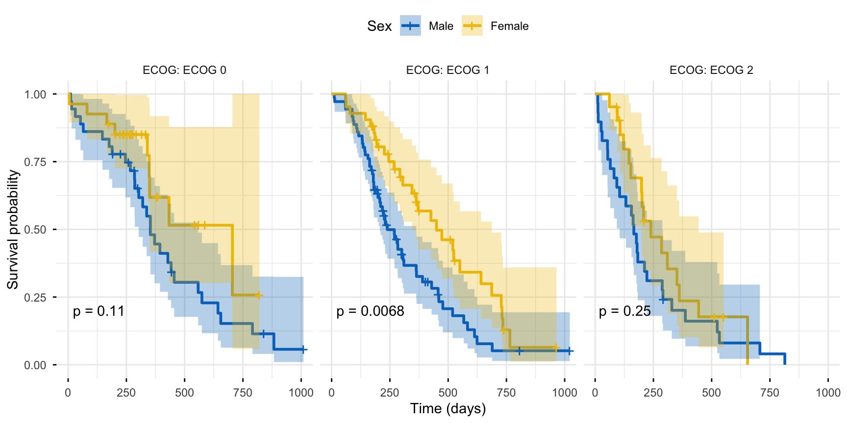
The stratified test compares groups within strata, so the matching figure shows the group curves in a separate panel per stratum. survminer’s ggsurvplot_facet() does exactly that. We drop the lone ECOG-3 patient and the one missing score so each panel has enough patients to draw, then facet by ECOG and print the within-stratum log-rank p-value on each panel:
library(survival)library(survminer)# Keep ECOG 0/1/2 (drop the single ECOG-3 patient and the one missing score)lung_ecog <- lung[!is.na(lung$ph.ecog) & lung$ph.ecog !=3, ]lung_ecog$ECOG <-factor(lung_ecog$ph.ecog,levels =c(0, 1, 2),labels =c("ECOG 0", "ECOG 1", "ECOG 2"))# Keep sex as the raw 1/2 codes and label the legend (the survminer-safe pattern)fit <-survfit(Surv(time, status) ~ sex, data = lung_ecog)ggsurvplot_facet( fit,data = lung_ecog,facet.by ="ECOG",pval =TRUE, # within-stratum log-rank p, on each panelconf.int =TRUE, # 95% confidence bandspalette ="jco", # colourblind-safe journal palettelegend.title ="Sex",legend.labs =c("Male", "Female"),xlab ="Time (days)",ylab ="Survival probability",ggtheme =theme_minimal())
Read the panels together: the female curve sits above the male curve in every ECOG stratum — the sex advantage is consistent across performance-score levels, which is exactly the condition the stratified test pools over. Notice the per-panel p-values (0.11, 0.0068, 0.25): each panel alone is underpowered because it holds only a slice of the patients, yet the stratified test pools all three into one comparison (χ² = 10.8, p = 0.001) with far more power than any single panel. That pooling is the value of stratifying over running separate within-group tests.
Report
Survival was compared between male and female patients with a log-rank test stratified by ECOG performance score on the NCCTG lung-cancer data (n = 227 after excluding one patient with a missing score). After adjusting for performance score, survival differed significantly between the sexes (χ²(1) = 10.8, p = 0.001), with females surviving longer; the result was unchanged from the unstratified test (χ²(1) = 10.3, p = 0.0013), indicating the sex difference was not confounded by performance score. Kaplan-Meier curves by sex within each ECOG stratum are shown in Figure 1.
NoteThe math behind the stratified log-rank test (optional)
The stratified log-rank test is a stratum-pooled version of the ordinary log-rank test. Within each stratum \(h\), at each event time you compute the observed minus expected events for group 1 and the variance, exactly as in the unstratified test — but separately per stratum. You then sum those contributions across strata before forming the statistic:
where \(O_{1h}\), \(E_{1h}\), and \(V_h\) are the observed events, expected events, and variance for group 1 within stratum\(h\), each accumulated over that stratum’s event times. Comparisons only ever happen among patients in the same stratum, so a factor that defines the strata cannot bias the group comparison. Under H₀ the statistic follows a chi-square distribution with (number of groups − 1) degrees of freedom — the strata are adjusted for, not tested, so they add no degrees of freedom. This is the Mantel-Haenszel idea applied to survival times.
Stratify or put it in a Cox model?
Stratifying and adjusting in a Cox model both control for a factor — they answer slightly different questions:
TipStratify vs. adjust
Stratified log-rank / stratified Cox — + strata(factor). Use when the factor is a nuisance confounder you want to remove, not estimate, and especially when its effect on survival may be non-proportional (the strata get their own baseline hazard, no proportional-hazards assumption on the stratifier). You get a p-value (and, in Cox, the group HR) adjusted for the factor — but no estimate for the factor itself.
Cox with the factor as a covariate — ~ group + factor. Use when you also want the factor’s own hazard ratio, or when it is continuous (age) — you cannot stratify on a continuous variable without binning it. Assumes proportional hazards for the factor.
Rule of thumb: a handful of categorical nuisance factors with possibly non-proportional effects → stratify; a factor whose effect size you care about, or a continuous one → covariate in Cox.
Try it live
Run the stratified log-rank test yourself — change the stratifier, or compare the stratified and unstratified results. The sandbox boots on first Run.
🟢 With an AI agent
Ask Prova“compare survival between my treatment groups while adjusting for study center with a stratified log-rank test, tell me in plain words whether stratifying changes the result, and draw the Kaplan-Meier curves faceted by center” — it answers with survival + survminer code you can run on your own data. The runtime is the judge.Ask Prova →
Common issues
Too many strata — the test gets unstable or “deletes” most of your data. Each level of each stratifying factor (and each combination, if you stratify on several) is a separate stratum, and a stratum with no events in one group contributes nothing. Stratify on all of stage, center, ECOG, and age band and you can end up with dozens of near-empty strata and a flaky χ². Keep to the one or two factors that are genuinely confounding; check stratum sizes with table(factor1, factor2, group) and aim for a reasonable number of events (not just patients) per stratum.
A missing stratifier value drops the patient.survdiff(... + strata(ph.ecog)) reports 1 observation deleted due to missingness because a patient with no ph.ecog has no stratum. If missingness is more than a few percent, that quietly shrinks your sample and can bias the result — decide deliberately (complete-case, an explicit “Missing” stratum via addNA(), or imputation) rather than letting rows vanish silently.
You stratified, but you actually wanted the factor’s effect.strata()removes the factor — it returns no hazard ratio or p-value for the stratifier. If you want the factor’s own effect (or it is continuous), put it in a Cox model as a covariate (~ group + factor) instead of in strata().
Frequently asked questions
NoteWhat is a stratified log-rank test used for?
A stratified log-rank test compares the survival of two or more groups while controlling for a prognostic factor — for example, comparing two treatments while adjusting for study center, disease stage, or performance score. It runs the log-rank comparison within each level of the factor and pools the results, so a factor that is unevenly distributed across the groups (a confounder) cannot bias the comparison. It is the standard analysis when a trial’s randomization was stratified by that factor.
NoteHow do I run a stratified log-rank test in R?
Use survdiff() with strata(): survdiff(Surv(time, status) ~ group + strata(factor), data = data). The grouping variable you compare goes on the left of + strata(); the confounder you adjust for goes insidestrata(). The output is a chi-square statistic and a p-value for the group difference, adjusted for the stratifying factor. The degrees of freedom equal the number of groups minus one — stratifying does not add degrees of freedom.
NoteWhen should I stratify versus adjust for a covariate in a Cox model?
Stratify (+ strata(factor)) when the factor is a nuisance confounder you want to remove but not estimate, and especially when its effect may be non-proportional over time — each stratum gets its own baseline hazard. Adjust (~ group + factor in a Cox model) when you also want the factor’s own hazard ratio, or when the factor is continuous (you cannot stratify on a continuous variable without binning it). A stratified log-rank test and a stratified Cox model answer the same question for a binary group; only Cox returns the hazard ratio.
NoteHow do I know if stratifying changed my conclusion?
Run both tests and compare the chi-square and p-value. If they are similar, the group difference is not confounded by that factor and your unstratified result is robust. If they differ markedly — significant unstratified but not stratified (or vice versa) — the factor was confounding the comparison, and the stratified result is the one to report. Always inspect the Kaplan-Meier curves within strata too: stratifying assumes the group effect is in a consistent direction across strata.
NoteHow many stratification factors can I use?
As few as do the job — usually one or two. Every level (and every combination across factors) is a separate stratum, and the data are split among them. Stratify on too many factors and you get sparse strata with too few events per cell, an unstable chi-square, and lost power. A rough guide is to keep enough events (not just patients) in each group within each stratum; if you need to control for several factors at once, a Cox model with covariate adjustment is usually the better tool.
Test your understanding
ImportantPractice
Run it. In the live cell below, stratify the sex comparison by ph.ecog — fill the blank inside strata(). The unstratified test on the same data runs just above it. Do the two p-values lead to the same conclusion?
Interpret. An unstratified log-rank test of two arms gives p = 0.04; stratified by study center it gives p = 0.21. In plain words, what does that tell you, and which result do you report?
NoteHint
Fill the blank with ph.ecog — it goes insidestrata(), because it is the factor you adjust for, not the groups you compare. Compare the Chisq/p lines of the two tests: if both give p well below 0.05, stratifying did not change the conclusion (the sex effect is not confounded by ECOG).
NoteSolution
survdiff(Surv(time, status) ~ sex, data = lung)#> Chisq = 10.3 on 1 df, p = 0.0013 (unstratified)survdiff(Surv(time, status) ~ sex +strata(ph.ecog), data = lung)#> Chisq = 10.8 on 1 df, p = 0.001 (stratified — 1 row dropped for missing ph.ecog)
Both tests are clearly significant (p ≈ 0.001), so they lead to the same conclusion: females survive longer, and that difference is not confounded by performance score.
For question 2: the unstratified test (p = 0.04) was significant, but after adjusting for study center it is not (p = 0.21). Study center was a confounder — the apparent arm difference was largely explained by an imbalance in center. Report the stratified result (p = 0.21): there is no convincing evidence of a treatment difference once center is accounted for.
TipQuick check
A trial randomized treatment within disease-stage blocks (stratified randomization). For the primary survival comparison, should you use a stratified or an unstratified log-rank test?
NoteShow answer
Stratified, with strata(stage). The analysis should match the design: when randomization was stratified by a factor, the primary analysis stratifies on the same factor. This preserves the balance the design built in and gives valid inference; an unstratified test ignores the stratified structure of the randomization.
Conclusion
You can now run the stratified log-rank test in R to compare survival between groups while controlling for a confounder: put the groups on the left and the confounder inside strata() — survdiff(Surv(time, status) ~ group + strata(factor), data) — and read the chi-square, its degrees of freedom (groups − 1, not inflated by the strata), and the p-value. The key move is to compare it with the unstratified test: if they agree, your comparison is robust to that factor; if they diverge, the factor was confounding and the stratified result is the one to trust. On the lung data, adjusting the sex comparison for performance score left it essentially unchanged (χ² 10.3 → 10.8, p ≈ 0.001). Visualize it with survminer’s ggsurvplot_facet(), one panel per stratum. When you need the adjusted hazard ratio — or to control for a continuous factor — reach for the Cox model instead.
Related lessons
Log-rank test — the unstratified comparison this lesson builds on; start there if you have not run a basic log-rank test. · Cox proportional hazards model — adjust for covariates (continuous or categorical) and get the hazard ratio, including the stratified Cox model. · Weighted log-rank test — the alternative when survival curves cross (non-proportional hazards) rather than when a factor confounds the comparison.
Every result on this page was produced by the code shown, run at build time against a pinned R environment — edit any block and Run to reproduce it yourself.