MANOVA in R: Compare Groups on Several Outcomes at Once
One-way multivariate analysis of variance the modern way — test a grouping factor against two or more continuous outcomes together, check the multivariate assumptions, and follow up with univariate ANOVAs
Biostatistics
Learn to run a one-way MANOVA in R. Test whether groups differ on several continuous outcome variables simultaneously with car’s Manova() and Pillai’s trace, check the MANOVA assumptions — multivariate normality, multivariate outliers, multicollinearity, homogeneity of covariances (Box’s M) and of variances — then follow a significant result with univariate ANOVAs and pairwise comparisons, with the p-values on the plot.
Published
June 23, 2026
Modified
July 12, 2026
TipKey takeaways
A one-way MANOVA (multivariate analysis of variance) tests whether groups differ across two or more continuous outcomes at once, instead of running a separate ANOVA per outcome.
Fit it with lm(cbind(y1, y2) ~ group) then car::Manova(); read Pillai’s trace (the robust default, best when assumptions are shaky or the design is unbalanced).
MANOVA adds multivariate assumptions: multivariate normality (mshapiro_test()), no multivariate outliers (Mahalanobis distance), moderate correlation between outcomes (no multicollinearity), and homogeneity of covariance matrices (Box’s M test).
A significant MANOVA is followed up with a univariate one-way ANOVA per outcome (Bonferroni-adjusted α), then pairwise comparisons to see which groups differ on which outcome.
Plot all outcomes together (a merged box plot) with the comparison p-values on it.
Introduction
A one-way MANOVA extends the one-way ANOVA to several outcome variables measured together. Instead of asking “do the groups differ on this score?” it asks “do the groups differ on the combination of these scores?” — testing a single grouping factor against a vector of continuous outcomes.
Use it when your outcomes measure different facets of one cohesive theme — several exam scores for overall academic performance, or several flower measurements for plant size — and you want one test of the joint difference rather than many separate ANOVAs (which inflate the error rate). The classic scenario: do iris species differ on the combination of Sepal.Length and Petal.Length? This lesson runs the full workflow with rstatix and car, using the built-in iris data.
Note
One-way MANOVA hypotheses.H₀: the group mean vectors are equal (the groups do not differ on the combined outcomes). Hₐ: at least one group’s mean vector differs. MANOVA builds a linear combination of the outcomes and compares its group means.
The data: two flower measurements by species
We use the built-in iris dataset, keeping two outcomes — Sepal.Length and Petal.Length — and the grouping factor Species (setosa, versicolor, virginica, 50 each):
MANOVA assumes adequate sample size (n per group > number of outcomes — here 50 > 2 ✓), independent observations, no multivariate outliers, multivariate normality, moderate (not excessive) correlation between outcomes, a linear relationship between the outcomes within each group, and homogeneity of covariance matrices.
Univariate outliers
First, check each outcome for extreme values within each group with identify_outliers() (an empty result means none):
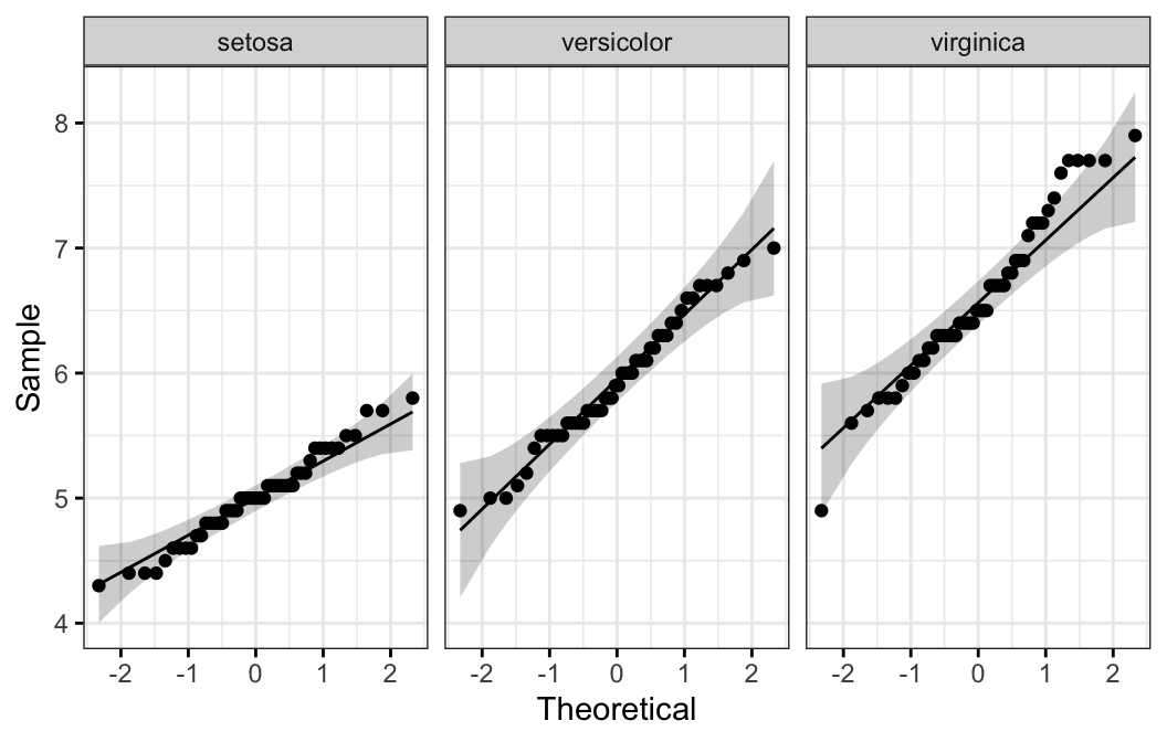
Both outcomes are normal in every group (p > 0.05), and mshapiro_test() is non-significant (p = 0.86) — multivariate normality holds. Back the test with a Q-Q plot per group:
The outcomes correlate at r = 0.87 (p < 0.0001) — high but below 0.9, so acceptable.
Check linearity assumption
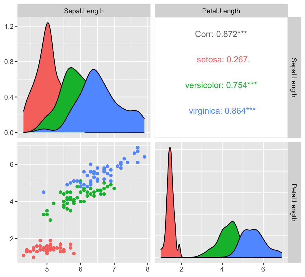
MANOVA builds a linear combination of the outcomes, so it assumes a linear relationship between the outcome variables within each group — a curved relationship would distort the multivariate test. Check it visually with a scatterplot matrix per group, using ggpairs() from the GGally package and colouring the points by species:
The off-diagonal panel plots Sepal.Length against Petal.Length for each species: within every group the points fall along a straight line with no curved or bent pattern, so the linearity assumption holds. (The upper panel prints the per-group correlations too — these vary in strength, but linearity is about the shape of each cloud, not how tight it is.)
If instead a group’s cloud were curved or U-shaped, the relationship would be non-linear. In that case, transform or remove the offending outcome variable, or run the MANOVA anyway and accept that you lose some statistical power.
Homogeneity of covariance matrices — Box’s M
Box’s M is the multivariate analogue of equal variances. It is very sensitive, so judge it at α = 0.001:
# A tibble: 1 × 4
  statistic  p.value parameter method
      <dbl>    <dbl>     <dbl> <chr>
1      58.4 9.62e-11         6 Box's M-test for Homogeneity of Covariance Matri…
Box’s M is significant (p < 0.001), so the covariance matrices are not homogeneous. With a balanced design (50 per group) this is not fatal — but it is the reason to report Pillai’s trace, the robust statistic, rather than Wilks’ lambda.
Homogeneity of variances — Levene’s test
For each outcome separately, reshape to long form with base R, then Levene’s test per outcome:
Levene’s test is significant for both outcomes — variances are not equal across species, which (with Box’s M) again points to Pillai’s trace and to Games-Howell for the post-hoc step.
Run the MANOVA
Fit a multivariate linear model with cbind() on the left, then Manova() with Pillai’s trace:
Type II MANOVA Tests: Pillai test statistic
        Df test stat approx F num Df den Df    Pr(>F)
Species  2    0.9885   71.829      4    294 < 2.2e-16 ***
---
Signif. codes:  0 '***' 0.001 '**' 0.01 '*' 0.05 '.' 0.1 ' ' 1
There is a statistically significant difference between species on the combined outcomes, F(4, 294) = 71.83, p < 0.0001 — species differ on the sepal-length/petal-length combination.
Tip
Which multivariate statistic?Manova() offers Pillai, Wilks, Hotelling-Lawley and Roy. Wilks’ lambda is the common default, but Pillai’s trace is more robust and is preferred when the design is unbalanced or Box’s M is significant (our case) — so we report Pillai.
Post-hoc: which outcomes, which groups
A significant MANOVA is decomposed into a univariate one-way ANOVA per outcome (Bonferroni-adjusted to α = 0.05 / 2 = 0.025 for two outcomes), then pairwise comparisons. Because variances are unequal, use the Games-Howell test:
Both outcomes differ significantly by species — Sepal.LengthF(2, 147) = 119 and Petal.LengthF(2, 147) = 1180 (both p < 0.0001) — and every pairwise species comparison is significant for each outcome.
Plot it with the p-values
The reporting figure overlays the pairwise comparisons on the merged box plot, with the MANOVA result in the subtitle (built with create_test_label()):
library(rstatix)library(ggpubr)iris2 <-data.frame(id =1:nrow(iris), iris[, c("Sepal.Length", "Petal.Length", "Species")])long <-data.frame(Species =rep(iris2$Species, 2),variables =rep(c("Sepal.Length", "Petal.Length"), each =nrow(iris2)),value =c(iris2$Sepal.Length, iris2$Petal.Length))pwc <- long %>%group_by(variables) %>%games_howell_test(value ~ Species) %>%add_xy_position(x ="Species")test.label <-create_test_label(description ="MANOVA", statistic.text =quote(italic("F")),statistic =71.83, p ="<0.0001", parameter ="4,294",type ="expression", detailed =TRUE)ggboxplot( iris2, x ="Species", y =c("Sepal.Length", "Petal.Length"),merge =TRUE, palette ="jco") +stat_pvalue_manual( pwc, hide.ns =TRUE, tip.length =0,step.increase =0.1, step.group.by ="variables", color ="variables" ) +labs(subtitle = test.label, caption =get_pwc_label(pwc, type ="expression"))
Report
A one-way MANOVA was performed to determine the effect of iris species on sepal length and petal length. There was a statistically significant difference between species on the combined dependent variables, F(4, 294) = 71.83, p < 0.0001 (Pillai’s trace). Follow-up univariate ANOVAs (Bonferroni-adjusted α = 0.025) showed a significant difference in sepal length, F(2, 147) = 119, and petal length, F(2, 147) = 1180 (both p < 0.0001). All pairwise comparisons between species were significant for each outcome.
NoteThe math (optional)
Where ANOVA partitions a single sum of squares, MANOVA partitions matrices: a between-groups matrix \(H\) (hypothesis) and a within-groups matrix \(E\) (error). The multivariate statistics summarise the \(H\)-vs-\(E\) relationship through the eigenvalues \(\lambda_i\) of \(E^{-1}H\). Pillai’s trace is \(V = \sum_i \frac{\lambda_i}{1 + \lambda_i}\) — a bounded, robust measure of how much of the combined variation lies between groups. Each multivariate statistic is converted to an approximate \(F\) for the p-value.
Try it live
Run a MANOVA on a fresh question — do iris species differ on the petal measurements (Petal.Length and Petal.Width) together? Edit the outcomes or the test statistic and re-run; the sandbox boots on first Run.
🟢 With an AI agent
Ask Prova“I have one grouping factor and several numeric outcomes — run a one-way MANOVA on my data, check the multivariate assumptions, and follow up a significant result with univariate ANOVAs” — it answers with rstatix + car code you can run on your own data, then helps you read Pillai’s trace and the follow-up tests. The runtime is the judge.Ask Prova →
Common issues
You ran a separate ANOVA per outcome instead of a MANOVA. Testing each outcome separately inflates the family-wise error rate and ignores the correlation between outcomes. Run the MANOVA first for the joint test; only then decompose into univariate ANOVAs (with a Bonferroni-adjusted α).
Box’s M is significant, so you used Wilks’ lambda. When Box’s M fails (unequal covariance matrices) or the design is unbalanced, Wilks’ lambda is not robust. Report Pillai’s trace instead — it is far less sensitive to the violation.
Your outcomes are almost perfectly correlated (r > 0.9). That is multicollinearity — the outcomes carry nearly the same information, which destabilises the MANOVA. Drop one of the redundant outcomes, or combine them into a single composite score.
Frequently asked questions
NoteWhat is the difference between ANOVA and MANOVA?
ANOVA tests a grouping factor against one continuous outcome; MANOVA tests it against two or more outcomes simultaneously, accounting for the correlation between them. MANOVA gives a single joint test (avoiding the inflated error rate of many separate ANOVAs) and can detect group differences that appear only in the combination of outcomes.
NoteShould I use Pillai’s trace or Wilks’ lambda?
Wilks’ lambda is the traditional default, but Pillai’s trace is more robust to violations of the homogeneity-of-covariance (Box’s M) assumption and to unbalanced designs. When Box’s M is significant — as in most real data — report Pillai’s trace. car::Manova() uses Pillai by default.
NoteWhat are the assumptions of MANOVA?
Adequate sample size (n per group greater than the number of outcomes), independent observations, no multivariate outliers (Mahalanobis distance), multivariate normality (mshapiro_test()), a linear relationship between outcomes, no multicollinearity (outcome correlations below 0.9), and homogeneity of covariance matrices (Box’s M). MANOVA is fairly robust to mild departures, especially with a balanced design.
NoteHow do I check the linearity assumption for MANOVA?
Draw a scatterplot matrix of the outcome variables for each group with ggpairs() from the GGally package (colour the points by group). The relationship between each pair of outcomes should look linear — a straight cloud with no curve — within every group. If a group shows a curved pattern, transform or remove that outcome variable, or run the MANOVA anyway and accept a loss of power.
NoteHow do I follow up a significant MANOVA?
Decompose it into a univariate one-way ANOVA for each outcome, using a Bonferroni-adjusted significance level (α divided by the number of outcomes). For each outcome that differs, run pairwise comparisons — Tukey HSD if variances are equal, Games-Howell if they are not — to see which groups differ.
Test your understanding
ImportantPractice
Run it. In the live cell, fit a one-way MANOVA of Sepal.Length and Sepal.Width by Species and report Pillai’s trace. Fill the blanks. Is the multivariate effect significant?
Conceptual. Box’s M is significant for your data. Which multivariate statistic should you report, and why?
NoteHint
Fill the outcomes as cbind(Sepal.Length, Sepal.Width) and the statistic as "Pillai". Read the Pr(>F) column. For question 2, recall which statistic is robust when the covariance matrices are unequal.
NoteSolution
library(rstatix); library(car)model <-lm(cbind(Sepal.Length, Sepal.Width) ~ Species, data = iris)Manova(model, test.statistic ="Pillai")#> Species effect is highly significant (p < 2e-16).
The multivariate effect is significant. For question 2: report Pillai’s trace — it is the robust statistic, least affected by a significant Box’s M (unequal covariance matrices).
Box’s M / equal variances violated → report Pillai’s trace and use Games-Howell post-hoc.
Conclusion
You can now run a one-way MANOVA in R: fit lm(cbind(y1, y2) ~ group), test it with car::Manova() reporting Pillai’s trace, and check the multivariate assumptions — multivariate normality, multivariate outliers, multicollinearity and Box’s M. When the joint test is significant, decompose it into univariate ANOVAs (Bonferroni-adjusted) and pairwise comparisons to see which groups differ on which outcome, then put the comparisons on a merged box plot. MANOVA is the right tool whenever several outcomes measure one cohesive theme.
Every result on this page was produced by the code shown, run at build time against a pinned R environment — edit any block and Run to reproduce it yourself.