Chi-Square Test of Independence in R: Are Two Variables Associated?

Test whether two categorical variables are associated, measure how strong with Cramér’s V, and find which cells drive the association — chi-square the modern way

Learn to run the chi-square test of independence in R — test whether two categorical variables are associated from a contingency table. Compute it with rstatix chisq_test() and base chisq.test(), check the expected-counts assumption (Fisher’s exact test for small counts), measure the strength with Cramér’s V, and find the cells that drive the association with Pearson residuals and a corrplot.

TipKey takeaways

• The chi-square test of independence asks whether two categorical variables are associated — does one depend on the other? — from their contingency table (cross-tabulation of counts).
• Run it with chisq.test() (base R) or rstatix::chisq_test(); a small p-value means the variables are not independent (they are associated).
• Assumption: every expected cell count should be ≥ 5; for small counts use Fisher’s exact test instead.
• Measure how strong the association is with Cramér’s V (cramer_v()) — significance ≠ strength.
• Find which cells drive the association with Pearson residuals and the cell contribution %, visualized with corrplot.

Introduction

The chi-square (χ²) test of independence tests whether two categorical variables are associated. Given a contingency table — the cross-tabulation of how many observations fall into each combination of categories — it compares the observed counts to the counts you’d expect if the two variables were independent. A large gap means the variables are related.

The classic scenario: in couples, is the person who does a household task associated with the type of task? This lesson runs the full workflow with base R and rstatix on the housetasks data, then shows how to read which cells create the association.

Note

Chi-square independence hypotheses. H₀: the two variables are independent (no association). Hₐ: they are associated (not independent). A significant result rejects independence — but always report the strength (Cramér’s V), not just the p-value.

Tip

Independence vs homogeneity — same test. The chi-square test of independence (one sample, cross-classified by two variables) and the chi-square test of homogeneity (several groups compared on one categorical outcome) use the identical computation (chisq.test() on a two-way table) — they differ only in study design and interpretation. Everything here applies to both.

The data: a contingency table

We use the housetasks.raw dataset from datarium and cross-tabulate it into a contingency table with base R’s xtabs() — 13 household tasks × who does them (Partner1, Partner2, Jointly, Alternating):

data("housetasks.raw", package = "datarium")
housetasks.xtab <- xtabs(~ tasks + status, data = housetasks.raw)
housetasks.xtab

            status
tasks        Partner1 Alternating Parter2 Jointly
  Laundry         156          14       2       4
  Main_meal       124          20       5       4
  Dinner           77          11       7      13
  Breakfeast       82          36      15       7
  Tidying          53          11       1      57
  Dishes           32          24       4      53
  Shopping         33          23       9      55
  Official         12          46      23      15
  Driving          10          51      75       3
  Finances         13          13      21      66
  Insurance         8           1      53      77
  Repairs           0           3     160       2
  Holidays          0           1       6     153

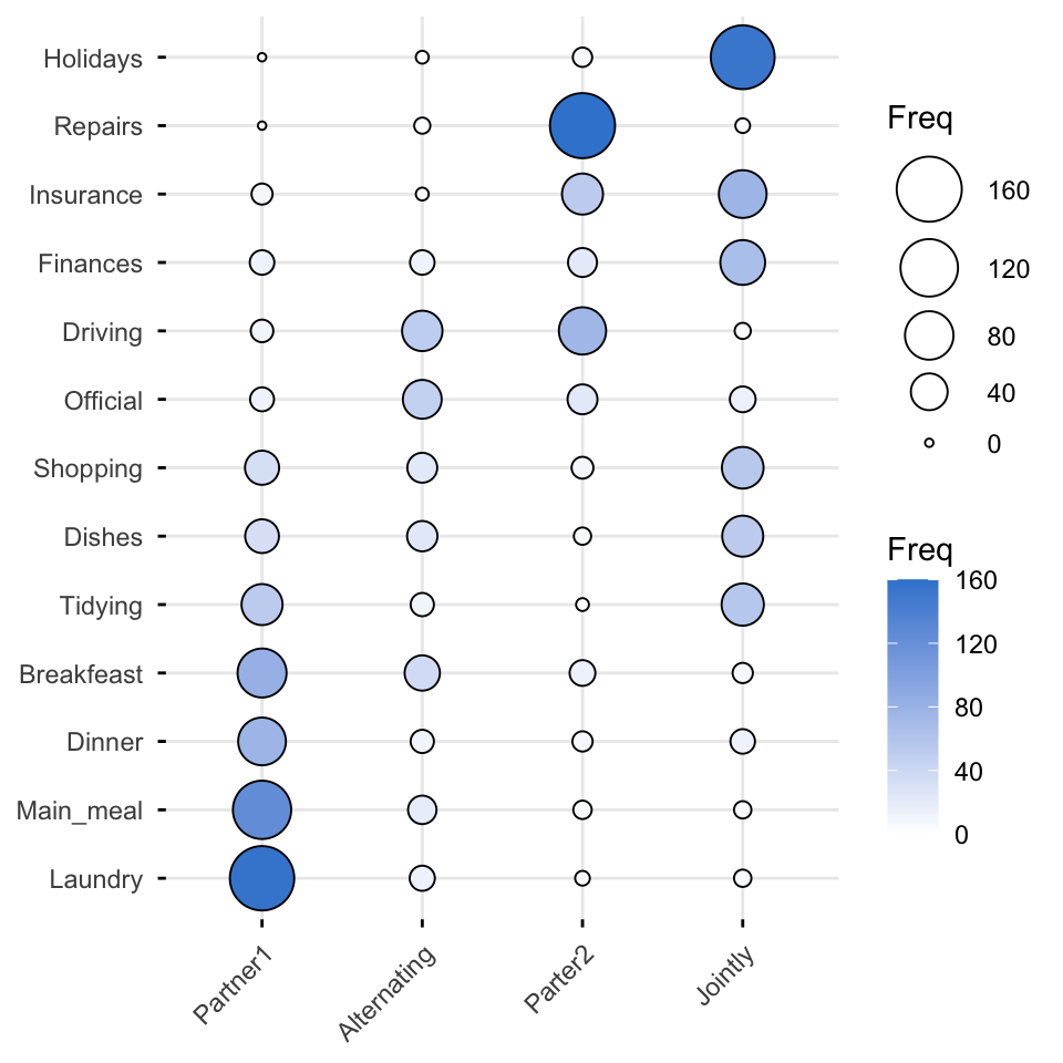
A balloon plot shows the table — bigger dots are bigger counts:

library(ggpubr)

data("housetasks.raw", package = "datarium")
housetasks.df <- as.data.frame(xtabs(~ tasks + status, data = housetasks.raw))

ggballoonplot(housetasks.df, x = "status", y = "tasks", size = "Freq", fill = "Freq") +
  gradient_fill(c("white", "#3a86d4"))

Run the chi-square test

With base R

chisq.test() takes the contingency table:

data("housetasks.raw", package = "datarium")
housetasks.xtab <- xtabs(~ tasks + status, data = housetasks.raw)

chisq <- chisq.test(housetasks.xtab)
chisq

    Pearson's Chi-squared test

data:  housetasks.xtab
X-squared = 1944.5, df = 36, p-value < 2.2e-16

The tasks and the person who does them are significantly associated, χ²(36) = 1944.5, p < 2.2e-16 — the two variables are not independent.

With rstatix

rstatix::chisq_test() gives the same result in a tidy row:

library(rstatix)

data("housetasks.raw", package = "datarium")
housetasks.xtab <- xtabs(~ tasks + status, data = housetasks.raw)

housetasks.xtab %>% chisq_test()

# A tibble: 1 × 6
      n statistic     p    df method          p.signif
* <int>     <dbl> <dbl> <int> <chr>           <chr>   
1  1744     1944.     0    36 Chi-square test ****    

Check the assumption: expected counts ≥ 5

The chi-square approximation is reliable only when every expected cell count is at least 5. Extract the expected counts from the test:

data("housetasks.raw", package = "datarium")
housetasks.xtab <- xtabs(~ tasks + status, data = housetasks.raw)

round(chisq.test(housetasks.xtab)$expected, 1)

            status
tasks        Partner1 Alternating Parter2 Jointly
  Laundry        60.6        25.6    38.4    51.4
  Main_meal      52.6        22.3    33.4    44.7
  Dinner         37.2        15.7    23.6    31.5
  Breakfeast     48.2        20.4    30.6    40.9
  Tidying        42.0        17.8    26.7    35.6
  Dishes         38.9        16.5    24.7    33.0
  Shopping       41.3        17.5    26.2    35.0
  Official       33.0        14.0    21.0    28.0
  Driving        47.8        20.2    30.4    40.6
  Finances       38.9        16.5    24.7    33.0
  Insurance      47.8        20.2    30.4    40.6
  Repairs        56.8        24.0    36.0    48.2
  Holidays       55.0        23.3    35.0    46.7

All expected counts here are well above 5, so chi-square is valid. If some are below 5, use Fisher’s exact test instead (fisher.test()), which makes no large-sample approximation.

Effect size: how strong is the association?

A significant chi-square says the variables are associated; Cramér’s V says how strongly (0 = none, 1 = perfect):

library(rstatix)

data("housetasks.raw", package = "datarium")
housetasks.xtab <- xtabs(~ tasks + status, data = housetasks.raw)

cramer_v(housetasks.xtab)

[1] 0.6096284

Cramér’s V = 0.61 — a strong association between the task and who does it. Always report it: with large samples even a trivial association is “significant”, so the effect size is what tells you it matters.

Which cells drive the association?

A significant table doesn’t say where the association lives. Two tools answer that.

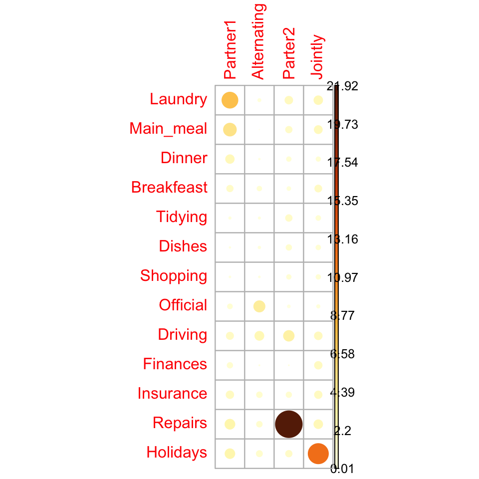
Pearson (standardized) residuals — (observed − expected) / √expected per cell. Large positive (blue) = more than expected (attraction); large negative (red) = fewer than expected (repulsion):

library(corrplot)

data("housetasks.raw", package = "datarium")
chisq <- chisq.test(xtabs(~ tasks + status, data = housetasks.raw))

corrplot(chisq$residuals, is.cor = FALSE)

Cell contribution % — each cell’s share of the total χ². The biggest contributors are the cells most responsible for the association:

library(corrplot)

data("housetasks.raw", package = "datarium")
chisq <- chisq.test(xtabs(~ tasks + status, data = housetasks.raw))

contrib <- 100 * chisq$residuals^2 / chisq$statistic
corrplot(contrib, is.cor = FALSE)

The top contributors are Repairs/Partner2 (≈ 22%), Holidays/Jointly (≈ 12%), Laundry/Partner1 (≈ 8%) and Main_meal/Partner1 (≈ 5%) — together ≈ 47% of the χ². So the association is mostly: repairs are a Partner2 job, holidays are decided jointly, and laundry/meals fall to Partner1.

Report

A chi-square test of independence found a statistically significant association between household task and who performs it, χ²(36) = 1944.5, p < 0.001, with a strong effect size (Cramér’s V = 0.61). Analysis of the cell contributions showed the association was driven mainly by Repairs being done by Partner2 and Holidays being decided jointly.

NoteThe math (optional)

The statistic sums the squared standardized gap between observed and expected counts over all cells: \(\chi^2 = \sum_{ij} \dfrac{(O_{ij} - E_{ij})^2}{E_{ij}}\), where the expected count under independence is \(E_{ij} = \dfrac{R_i\,C_j}{N}\) (row total × column total ÷ grand total). It is compared to a chi-square distribution with \((r-1)(c-1)\) degrees of freedom. Cramér’s V rescales it to 0–1: \(V = \sqrt{\chi^2 / [N\,(k-1)]}\), where \(k\) is the smaller of the number of rows and columns.

Try it live

Run the chi-square test on a built-in table — is hair colour associated with eye colour? Edit it and re-run; the sandbox boots on first Run.

🟢 With an AI agent

Ask Prova “I have two categorical variables — test whether they’re associated with a chi-square test, tell me the effect size, and which cells drive it” — it answers with rstatix code you can run on your own contingency table. The runtime is the judge. Ask Prova →

Common issues

Some expected counts are below 5. The chi-square approximation is then unreliable — switch to Fisher’s exact test (fisher.test()), which is exact for small counts.

You reported significance but not strength. With a large sample, chi-square is significant even for a tiny association. Always report Cramér’s V so readers know whether the association is large enough to matter.

You passed raw data instead of a table. chisq.test() wants the contingency table (table() or xtabs() of the two variables), not the raw data frame — or pass the two factor columns directly, chisq.test(x, y).

Frequently asked questions

NoteWhat is the chi-square test of independence?

It tests whether two categorical variables are associated — whether the distribution of one depends on the other — by comparing the observed cell counts in their contingency table to the counts expected if the variables were independent. A significant result means the variables are associated.

NoteWhat is the difference between the chi-square test of independence and homogeneity?

They use the same computation (chisq.test() on a two-way table) and differ only in study design. Independence: one sample cross-classified by two variables (are they related?). Homogeneity: several independent groups compared on one categorical outcome (do the groups have the same distribution?). The R code and interpretation of the p-value are identical.

NoteWhat are the assumptions of the chi-square test?

Independent observations, a sufficiently large sample, and — the key one — every expected cell count ≥ 5 (some allow a few cells between 1 and 5). When expected counts are too small, the chi-square approximation breaks down and you should use Fisher’s exact test.

NoteWhat effect size goes with a chi-square test?

Cramér’s V (0 to 1) for any size table, or the phi coefficient for a 2×2 table. Compute it with rstatix::cramer_v(). Report it alongside the p-value, because a significant chi-square says only that an association exists, not how strong it is.

Test your understanding

ImportantPractice

1. Run it. In the live cell, test whether hair colour and eye colour are associated in HairEyeColor, and report Cramér’s V. Fill the blank. Is the association significant, and how strong?
2. Conceptual. Your chi-square is significant with a huge sample but Cramér’s V = 0.03. What do you conclude?

NoteHint

Fill the blank with cramer_v. For question 2, recall that significance and strength are different things, especially with large n.

NoteSolution

tab <- margin.table(HairEyeColor, c(1, 2))
chisq_test(tab)   #> p < 0.0001 — associated
cramer_v(tab)     #> ~0.28 — a moderate association

For question 2: a significant test with Cramér’s V = 0.03 means the variables are technically associated but the association is negligibly weak — the significance is an artefact of the large sample. Report the tiny effect size and treat the variables as practically independent.

TipWhich test when?

• Two categorical variables, large counts → chi-square test of independence (this lesson).
• Two categorical variables, small expected counts → Fisher’s exact test.
• One categorical variable vs expected proportions → chi-square goodness-of-fit.
• Paired categorical data → McNemar (2×2) or Cochran’s Q (≥3).

Conclusion

You can now run the chi-square test of independence in R: cross-tabulate with xtabs(), test with chisq.test() / rstatix::chisq_test(), check the expected-counts ≥ 5 assumption (Fisher’s exact test otherwise), report the strength with Cramér’s V, and use Pearson residuals + cell contributions to pinpoint which categories drive the association. It is the workhorse test for any two-way table of counts — and the homogeneity test is the very same computation.

Related lessons

• Fisher’s exact test in R — the small-counts alternative. · Chi-square goodness-of-fit in R — one variable vs expected proportions. · Odds ratio & relative risk in R — effect sizes for a 2×2 table. · Proportion z-tests in R — comparing two proportions (≡ a 2×2 chi-square).
• Go further: Categorical data analysis · Biostatistics

Was this page helpful?

Prove you can do it. Master the whole Categorical Analysis in R series — track your path, build projects, and earn a certificate.

Start free →

Go Pro — unlimited Prova on your own data and a verifiable certificate that proves the skill.

from $15/mo billed yearly

Go Pro →

✓ You're Pro — keep going. The runtime is the judge.

Ready to level up?

Try this on your own data with Prova — the runtime is the judge.Open Prova →

Get new R & Python lessons by email

Practical, reproducible, no spam. Unsubscribe anytime.

Double opt-in. We never share your email.

Share this pageXLinkedInRedditHN

Note

Every result on this page was produced by the code shown, run at build time against a pinned R environment — edit any block and Run to reproduce it yourself.