Testing the Proportional Hazards Assumption in R (cox.zph, Schoenfeld)

Q: How do I test the proportional hazards assumption in R?

Fit your Cox model with coxph(), then pass it to cox.zph(): test.ph <- cox.zph(res.cox). It returns a per-covariate test plus a GLOBAL test, each based on the scaled Schoenfeld residuals. A non-significant p-value (≥ 0.05) supports proportional hazards; a significant one (< 0.05) means it is violated. Visualize it with ggcoxzph(test.ph) from survminer.

Q: What does it mean if cox.zph is significant?

A significant cox.zph() p-value (< 0.05) means the hazard ratio for that covariate is not constant over time — the proportional-hazards assumption is violated, so the single HR the Cox model reports is a misleading time-average. Look at the ggcoxzph() panel to see the shape of the time trend, then fix it by stratifying the covariate, adding a time-varying coefficient (tt()) or time interaction, or using a weighted log-rank test.

Q: What are Schoenfeld residuals?

Schoenfeld residuals are, at each event time, the difference between the covariate value of the patient who had the event and the average covariate value among everyone still at risk — one residual per event, per covariate. The scaled Schoenfeld residuals track the time-varying coefficient β(t), so under proportional hazards a plot of them against time should be flat. A systematic trend means the effect changes over time, i.e. PH is violated. That is exactly what cox.zph() tests and ggcoxzph() plots.

Q: How do I check for influential observations in a Cox model?

Use survminer’s ggcoxdiagnostics(). type = "dfbeta" shows how much each coefficient would change if each observation were deleted — a value large relative to the coefficient flags an influential patient. type = "deviance" shows deviance residuals, which should be roughly symmetric about zero; very large or small values are poorly-predicted outliers worth inspecting.

Q: How do I check whether a continuous covariate is linear in a Cox model?

Plot martingale residuals against the covariate with ggcoxfunctional() and look at the lowess smooth: roughly straight means a linear form is fine; a clear bend means you should transform the covariate (e.g. log(), a spline, or polynomial terms). This matters only for continuous covariates — categorical ones can’t be non-linear.

Check whether your Cox model’s hazard ratios are constant over time — cox.zph, scaled Schoenfeld residuals with ggcoxzph, influence and non-linearity diagnostics, and what to do when PH fails

Biostatistics

Validate a Cox proportional hazards model in R. Test the proportional-hazards (PH) assumption with cox.zph and the scaled Schoenfeld residual plot ggcoxzph, check for influential observations with ggcoxdiagnostics (dfbeta and deviance residuals), test the functional form of continuous covariates with martingale residuals, and learn the remedies when PH is violated — stratification, time-varying coefficients, and time interactions.

Published

June 25, 2026

Modified

July 7, 2026

Key takeaways

The Cox model rests on one assumption: proportional hazards (PH) — the hazard ratio between any two patients stays constant over time. If a covariate’s effect grows, shrinks, or reverses over follow-up, the single hazard ratio is misleading and must be fixed.
Test PH with cox.zph() — it correlates each covariate’s scaled Schoenfeld residuals with time. Non-significant (p ≥ 0.05) = PH holds; significant (p < 0.05) = PH violated. It reports a per-covariate test and a GLOBAL test for the whole model.
Visualize it with survminer’s ggcoxzph() — scaled Schoenfeld residuals vs. time. A flat smoothing line supports PH; a systematic trend signals a violation.
Also check influential observations (ggcoxdiagnostics(fit, type = "dfbeta") / "deviance") and the functional form of continuous covariates (martingale residuals via ggcoxfunctional()).
When PH fails, don’t abandon the model — stratify the offending covariate, add a time-varying coefficient (tt()) or a time interaction, or use a weighted log-rank test.

Introduction

You have fit a Cox proportional hazards model on your survival data and read off the hazard ratios — female sex cuts the hazard of death by ~42%, a worse ECOG score raises it by ~59%. Clean numbers, a tidy forest plot. But there is a catch: every one of those hazard ratios assumes the effect is constant over the whole follow-up. That is the proportional-hazards (PH) assumption, and it is the single thing a Cox model can get wrong in a way that quietly invalidates the result.

Picture a trial where a treatment helps early but its benefit fades after a year (or kicks in late, as immunotherapy often does). The survival curves cross or converge — the hazard ratio is not constant — and the one HR the model prints is a misleading time-average that hides the real story. Used inappropriately, a Cox model gives confident, wrong conclusions. So before you trust a hazard ratio, test the assumption that produced it.

This lesson walks the full diagnostic workflow for a Cox model in R, using survival (the tests) and survminer (the publication-grade diagnostic plots), on the same NCCTG lung-cancer model from the Cox lesson. You will learn to:

test proportional hazards with cox.zph() and read its per-covariate and global tests;
plot scaled Schoenfeld residuals with the signature ggcoxzph() figure;
find influential observations with ggcoxdiagnostics() (dfbeta and deviance residuals);
test the functional form of continuous covariates with martingale residuals;
and fix a PH violation when you find one.

What we are testing

We check whether the Cox model is an adequate representation of the data by examining its residuals:

Schoenfeld residuals → the proportional-hazards assumption (constant HR over time).
dfbeta / deviance residuals → influential observations (a few points distorting the fit).
Martingale residuals → the functional form of continuous covariates (linear vs. non-linear).

H₀ (for PH): the hazard ratio is constant over time (residuals are independent of time). Hₐ: the hazard ratio changes over time (a trend in the residuals). A significant test rejects PH.

The data and the model

We reuse lung, the North Central Cancer Treatment Group dataset that ships with the survival package (228 advanced lung-cancer patients), and the same multivariate Cox model from the Cox lesson: survival on age, sex, and ECOG performance score. Load the package — lung attaches automatically — and fit the model:

library(survival)

res.cox <- coxph(Surv(time, status) ~ age + sex + ph.ecog, data = lung)
res.cox

Call:
coxph(formula = Surv(time, status) ~ age + sex + ph.ecog, data = lung)

             coef exp(coef)  se(coef)      z        p
age      0.011067  1.011128  0.009267  1.194 0.232416
sex     -0.552612  0.575445  0.167739 -3.294 0.000986
ph.ecog  0.463728  1.589991  0.113577  4.083 4.45e-05

Likelihood ratio test=30.5  on 3 df, p=1.083e-06
n= 227, number of events= 164 
   (1 observation effacée parce que manquante)

A reminder of the coding: status is 1 = censored / 2 = dead, sex is 1 = male / 2 = female, ph.ecog is the ECOG performance score (0 = fully active, higher = more impaired). This is the fitted object we now put through its diagnostics.

Test the proportional-hazards assumption with `cox.zph()`

The PH assumption can be checked with a statistical test and a graphical diagnostic, both built on the scaled Schoenfeld residuals. The idea is simple: under proportional hazards, the Schoenfeld residuals are independent of time. A residual pattern that drifts with time is evidence the hazard ratio is not constant — i.e. PH is violated.

The function cox.zph() (in the survival package) does exactly this. For each covariate it correlates the scaled Schoenfeld residuals with (transformed) time, and it adds a GLOBAL test for the model as a whole. Pass it the fitted coxph object:

library(survival)

res.cox <- coxph(Surv(time, status) ~ age + sex + ph.ecog, data = lung)

test.ph <- cox.zph(res.cox)
test.ph

        chisq df    p
age     0.188  1 0.66
sex     2.305  1 0.13
ph.ecog 2.054  1 0.15
GLOBAL  4.464  3 0.22

Read the output:

Each row is one covariate; the last row, GLOBAL, tests the whole model.
The decision rule is the same everywhere: p ≥ 0.05 → PH is supported (no time trend); p < 0.05 → PH is violated for that covariate.
Here every per-covariate p-value is comfortably large — age p = 0.66, sex p = 0.13, ph.ecog p = 0.15 — and the GLOBAL test is p = 0.22 (χ² = 4.46 on 3 df). None is significant, so the proportional-hazards assumption is supported for this model: the hazard ratios can be read as constant over time.

How to phrase the verdict

The proportional-hazards assumption is supported by a non-significant relationship between the scaled Schoenfeld residuals and time, and refuted by a significant one. Always read the GLOBAL test (the whole model) together with the per-covariate tests (which covariate is the culprit).

The signature diagnostic: scaled Schoenfeld residuals (`ggcoxzph()`)

The number is reassuring; the picture is what you put in a paper. survminer’s ggcoxzph() draws, for each covariate, the scaled Schoenfeld residuals against transformed time, with a smoothing spline and a ±2-standard-error band. Pass it the cox.zph object you just made:

library(survival)
library(survminer)

res.cox <- coxph(Surv(time, status) ~ age + sex + ph.ecog, data = lung)
test.ph <- cox.zph(res.cox)

ggcoxzph(test.ph)

A survminer ggcoxzph diagnostic with one panel per covariate (age, sex, ECOG score), each showing scaled Schoenfeld residuals plotted against transformed survival time. In every panel the solid smoothing spline is roughly flat and horizontal, staying within the dashed plus-or-minus two-standard-error band, indicating no systematic time trend and supporting the proportional-hazards assumption.

How to read it (the one skill that matters here):

The solid line is a smoothing spline through the residuals; the dashed lines are a ±2 SE band.
A flat, horizontal line (no trend with time) means the effect is constant → PH holds.
A systematic slope or curve — the line drifting up or down across follow-up — means the hazard ratio is changing over time → PH is violated for that covariate.
In all three panels the spline is essentially flat and stays inside the band, so there is no pattern with time: the assumption is supported for age, sex (the two-level factor accounts for the two residual bands), and ph.ecog. This matches the non-significant cox.zph() p-values exactly.

A second graphical check for categorical covariates

For a categorical predictor you can also plot log(−log(S(t))) against time (or log-time) for each group and look for parallel curves — parallel lines support PH, crossing or converging lines flag a violation. The Schoenfeld-residual approach above is the general workhorse (it handles continuous covariates too), so it is what we lead with.

Influential observations (`ggcoxdiagnostics()`)

A second question for any model: is the fit being driven by a few unusual patients? Two residual types answer it, both via survminer’s ggcoxdiagnostics():

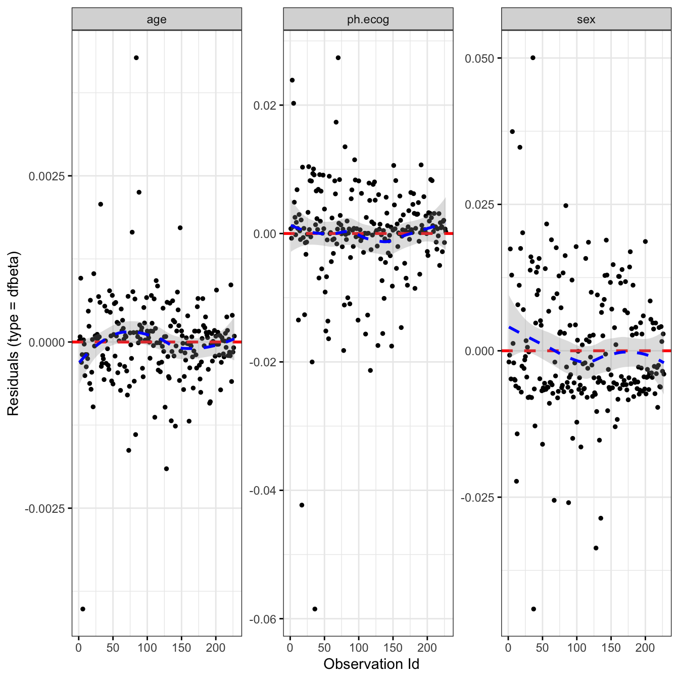
type = "dfbeta" plots the estimated change in each regression coefficient when each observation is deleted in turn — a large dfbeta means dropping that one patient would move the coefficient a lot.
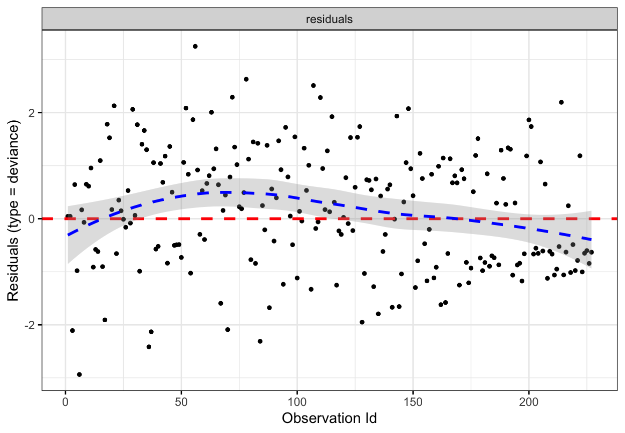
type = "deviance" plots deviance residuals, a symmetric transform of the martingale residuals.

dfbeta — how much each patient moves the coefficients

library(survival)
library(survminer)

res.cox <- coxph(Surv(time, status) ~ age + sex + ph.ecog, data = lung)

ggcoxdiagnostics(res.cox, type = "dfbeta", linear.predictions = FALSE)

A survminer ggcoxdiagnostics dfbeta plot with one panel per covariate (age, sex, ECOG score), each showing the change in that coefficient when each observation is deleted, plotted against observation index. The points scatter around zero with no single observation dominating, indicating no terribly influential patients.

Read it: compare the magnitude of the largest dfbeta values to the size of the coefficients themselves. Here a handful of points for age and ph.ecog are larger than the rest, but none is large relative to its coefficient — no single patient is terribly influential, so we don’t need to remove anyone. If one point dwarfed the others, you would inspect that patient and check whether the result depends on them.

Deviance residuals — who is poorly predicted

library(survival)
library(survminer)

res.cox <- coxph(Surv(time, status) ~ age + sex + ph.ecog, data = lung)

ggcoxdiagnostics(res.cox, type = "deviance", linear.predictions = FALSE)

A survminer ggcoxdiagnostics deviance-residual plot showing deviance residuals against observation index. The points are roughly symmetrically distributed about zero, with no extreme outliers, indicating the model predicts most patients reasonably well.

Read it: deviance residuals should be roughly symmetric about zero with a standard deviation near 1. Positive values flag patients who “died too soon” relative to the model’s prediction; negative values, those who “lived too long”; very large or small values are poorly-predicted outliers. The pattern here is fairly symmetric around zero with no extreme points — the model predicts most patients reasonably well.

Non-linearity: the functional form of continuous covariates (`ggcoxfunctional()`)

Cox regression assumes each continuous covariate enters linearly on the log-hazard scale — but age might act non-linearly (say, risk flat until 60, then rising). The standard check plots martingale residuals of a null model against the covariate and looks at the lowess (smooth) fit: it should be roughly linear. survminer’s ggcoxfunctional() does this; fit a small Cox model that includes the covariate in a few forms — age, log(age), sqrt(age) — and pass it in:

library(survival)
library(survminer)

cox.age <- coxph(Surv(time, status) ~ age + log(age) + sqrt(age), data = lung)

ggcoxfunctional(cox.age, data = lung)

A survminer ggcoxfunctional plot with three panels showing martingale residuals against age, log(age), and sqrt(age) from a null Cox model on the lung data, each with a lowess smoothing line. The smooths are close to linear with only a slight bend, indicating age can reasonably enter the model in linear form.

Read it: a straight lowess line means the covariate is well fit in that form; a clear bend means you should transform it (use log(age), a spline, or polynomial terms) instead of raw age. Non-linearity is only relevant for continuous covariates — it is not an issue for categorical ones like sex. Here the smooths are close to linear with only a slight bend, so entering age linearly is reasonable.

What to do when proportional hazards fails

When cox.zph() flags a covariate (p < 0.05) or its ggcoxzph() panel shows a clear trend, you don’t throw the model away — you account for the time-varying effect. The main remedies:

Stratify the offending covariate — coxph(Surv(time, status) ~ age + sex + strata(ph.ecog)) lets each stratum have its own baseline hazard, so PH no longer needs to hold for that variable. Best for a “nuisance” confounder you don’t need an effect estimate for (you lose its hazard ratio).
Add a time-varying coefficient — model the effect as a function of time, e.g. with tt(): coxph(Surv(time, status) ~ sex + tt(sex), tt = function(x, t, ...) x * log(t)), or split the follow-up at a cut-point and fit a separate HR per interval (an early vs late effect).
Add a covariate × time interaction — a step-function version of the above, giving an interpretable “the effect in the first 12 months vs. after”.
Use a weighted log-rank test (Fleming-Harrington) for the group comparison when curves cross — it up-weights early or late differences instead of assuming a constant ratio.

Pick the remedy by what’s violating

A categorical “nuisance” covariate violates PH → stratify it.
A treatment / key effect changes over time → a time-varying coefficient or time interaction (so you can report the early vs. late effect).
The group survival curves cross → consider a weighted log-rank test alongside the Cox model.

Report

The proportional-hazards assumption of the multivariate Cox model (age, sex, ECOG score) was assessed with scaled Schoenfeld residuals (cox.zph). There was no evidence of a violation for any covariate (age p = 0.66, sex p = 0.13, ECOG score p = 0.15) nor for the model as a whole (GLOBAL χ²(3) = 4.46, p = 0.22); the ggcoxzph residual plots showed no systematic trend with time. Influence diagnostics (dfbeta, deviance residuals) revealed no unduly influential observations, and martingale residuals supported a linear functional form for age. The proportional-hazards assumption was therefore considered satisfied.

The math behind Schoenfeld residuals (optional)

At each event time, the Schoenfeld residual for a covariate is the difference between the covariate value of the patient who had the event and the expected value over all patients still at risk:

\[ r_{ij} = x_{ij} - \bar{x}_{j}(t_i) \]

where \(x_{ij}\) is covariate \(j\) for the patient with an event at time \(t_i\), and \(\bar{x}_{j}(t_i)\) is the risk-set-weighted average of that covariate at \(t_i\). There is one residual per event (none for censored observations), per covariate.

Grambsch and Therneau showed that the scaled Schoenfeld residuals have an expected value that is approximately the time-varying coefficient \(\beta_j(t)\). So under proportional hazards \(\beta_j(t) = \beta_j\) is constant, and a plot of the scaled residuals against time should be flat. cox.zph() formalizes this by testing whether the residuals are correlated with time (a non-zero slope \(\Rightarrow\) a time-varying effect \(\Rightarrow\) PH violated). That is exactly the “flat line = good” rule you read off ggcoxzph().

Which diagnostic when?

Choosing your Cox diagnostic

Are the hazard ratios constant over time? → cox.zph() + ggcoxzph() (scaled Schoenfeld residuals) — the PH test, the main event.
Is a handful of patients driving the fit? → ggcoxdiagnostics(fit, type = "dfbeta") (influence on coefficients) and type = "deviance" (poorly-predicted outliers).
Does a continuous covariate enter linearly? → ggcoxfunctional() (martingale residuals).
PH is violated — now what? → stratify, time-varying coefficient (tt()), time interaction, or a weighted log-rank test.

Try it live

Test the assumption yourself — run cox.zph() and draw the ggcoxzph() panels. Try adding wt.loss to the model, or check a single covariate. The sandbox boots on first Run.

🟢 With an AI agent

Ask Prova “test the proportional hazards assumption of my Cox model with cox.zph and ggcoxzph, tell me in plain words whether it holds, and if it’s violated show me how to fix it” — it answers with survival + survminer code you can run on your own data. The runtime is the judge. Ask Prova →

Common issues

You read only the GLOBAL test, or only the per-covariate tests. Read both. A non-significant GLOBAL test with one significant covariate still means that covariate violates PH and needs attention; a significant GLOBAL with all-borderline covariates tells you something is off but not where. The GLOBAL test answers “is the model OK overall?”, the per-covariate rows answer “which variable is the problem?”.

A “significant” PH test on a huge sample isn’t always a real problem. With thousands of events, cox.zph() can flag a tiny, clinically irrelevant time trend as statistically significant. Always look at the ggcoxzph() plot: a residual line that is essentially flat but technically sloped is far less concerning than one that clearly drifts or reverses. Judge the magnitude and shape, not just the p-value.

A small sample makes the test noisy. With few events the scaled Schoenfeld residuals are noisy and the test has low power — a non-significant result is weak evidence PH holds, and a wide confidence band on the plot is expected. Pair the test with the plot and with clinical reasoning about whether the effect should change over time.

ggcoxfunctional() errors on the formula form. Newer survminer wants the fitted model, not a formula: fit cox.age <- coxph(Surv(time, status) ~ age + log(age) + sqrt(age), data = lung) first, then call ggcoxfunctional(cox.age, data = lung).

Frequently asked questions

How do I test the proportional hazards assumption in R?

Fit your Cox model with coxph(), then pass it to cox.zph(): test.ph <- cox.zph(res.cox). It returns a per-covariate test plus a GLOBAL test, each based on the scaled Schoenfeld residuals. A non-significant p-value (≥ 0.05) supports proportional hazards; a significant one (< 0.05) means it is violated. Visualize it with ggcoxzph(test.ph) from survminer.

What does it mean if cox.zph is significant?

A significant cox.zph() p-value (< 0.05) means the hazard ratio for that covariate is not constant over time — the proportional-hazards assumption is violated, so the single HR the Cox model reports is a misleading time-average. Look at the ggcoxzph() panel to see the shape of the time trend, then fix it by stratifying the covariate, adding a time-varying coefficient (tt()) or time interaction, or using a weighted log-rank test.

What are Schoenfeld residuals?

Schoenfeld residuals are, at each event time, the difference between the covariate value of the patient who had the event and the average covariate value among everyone still at risk — one residual per event, per covariate. The scaled Schoenfeld residuals track the time-varying coefficient β(t), so under proportional hazards a plot of them against time should be flat. A systematic trend means the effect changes over time, i.e. PH is violated. That is exactly what cox.zph() tests and ggcoxzph() plots.

How do I check for influential observations in a Cox model?

Use survminer’s ggcoxdiagnostics(). type = "dfbeta" shows how much each coefficient would change if each observation were deleted — a value large relative to the coefficient flags an influential patient. type = "deviance" shows deviance residuals, which should be roughly symmetric about zero; very large or small values are poorly-predicted outliers worth inspecting.

How do I check whether a continuous covariate is linear in a Cox model?

Plot martingale residuals against the covariate with ggcoxfunctional() and look at the lowess smooth: roughly straight means a linear form is fine; a clear bend means you should transform the covariate (e.g. log(), a spline, or polynomial terms). This matters only for continuous covariates — categorical ones can’t be non-linear.

Test your understanding

Practice

Run it. In the live cell below, fit a Cox model that adds wt.loss (weight loss) to the model, then test proportional hazards with cox.zph(). Fill the blank. Does wt.loss satisfy the PH assumption, and does the GLOBAL test?
Interpret. A cox.zph() GLOBAL test gives p = 0.004, with treatment p = 0.002 and all other covariates p > 0.3. Which assumption is violated, for which covariate, and name one appropriate remedy.

Hint

Fill the blank with wt.loss. Read each row’s p-value: p ≥ 0.05 means PH is supported for that covariate; check the GLOBAL row for the whole model. The ggcoxzph() panels should be flat if PH holds.

Solution

res.cox <- coxph(Surv(time, status) ~ age + sex + ph.ecog + wt.loss, data = lung)
test.ph <- cox.zph(res.cox)
test.ph
#> Every per-covariate p-value and the GLOBAL p-value are > 0.05 (non-significant),
#> so the proportional-hazards assumption is SUPPORTED for the model — including wt.loss.
#> The ggcoxzph() panels show flat smoothing lines, confirming no time trend.

For question 2: the proportional-hazards assumption is violated (GLOBAL p = 0.004 < 0.05), and the culprit is treatment (p = 0.002), since the other covariates are non-significant. The treatment effect is changing over time. One appropriate remedy: model it with a time-varying coefficient (tt()) or a treatment × time interaction so you can report the early vs. late effect (stratifying treatment would hide the very effect you care about). A weighted log-rank test is a reasonable companion for the group comparison.

Quick check

cox.zph() returns a GLOBAL p-value of 0.45, and every per-covariate p-value is above 0.3. What do you conclude?

Show answer

The proportional-hazards assumption is supported. All p-values are non-significant (≥ 0.05), so there is no evidence that any covariate’s hazard ratio changes over time — the Cox model’s hazard ratios can be read as constant over follow-up, and no remedy (stratification, time-varying coefficient) is needed. Confirm with the ggcoxzph() plot: the smoothing lines should be flat.

Conclusion

You can now validate a Cox proportional hazards model in R. Test the core assumption with cox.zph() — reading the per-covariate and GLOBAL tests, where a non-significant p-value supports PH — and see it with survminer’s ggcoxzph() scaled Schoenfeld residual plot, where a flat line means the hazard ratios hold steady over time. Round out the check with ggcoxdiagnostics() for influential observations (dfbeta, deviance) and ggcoxfunctional() for the functional form of continuous covariates. On the lung-cancer model, every diagnostic passed (GLOBAL p = 0.22), so the hazard ratios from the Cox lesson are trustworthy. And when a diagnostic does fail, you now know the fixes — stratify, a time-varying coefficient, a time interaction, or a weighted log-rank test — so a violation is a problem you solve, not a result you discard.

Reuse

CC BY-NC-SA 4.0

Citation

BibTeX citation:

@online{2026,
  author = {},
  title = {Testing the {Proportional} {Hazards} {Assumption} in {R}
    (Cox.zph, {Schoenfeld)}},
  date = {2026-06-25},
  url = {https://www.datanovia.com/learn/biostatistics/survival-analysis/testing-ph-assumptions},
  langid = {en}
}

For attribution, please cite this work as:

“Testing the Proportional Hazards Assumption in R (Cox.zph, Schoenfeld).” 2026. June 25. https://www.datanovia.com/learn/biostatistics/survival-analysis/testing-ph-assumptions.