Sample Size for Survival Analysis: How Many Events Do You Need?
Plan a time-to-event study the right way — why power depends on the number of events (not patients), the Schoenfeld events formula in R, and turning events into a patient count, accrual, and follow-up
Biostatistics
Design a time-to-event study before you collect data. Learn the one insight that governs survival power — it is driven by the number of EVENTS, not the number of patients — compute the required number of events for a log-rank or Cox comparison with the Schoenfeld formula in base R, convert events into a patient count given an expected event probability, and plan accrual, follow-up, dropout, and stratified (biomarker) design.
Published
June 26, 2026
Modified
July 7, 2026
TipKey takeaways
Survival power is driven by the number of EVENTS, not the number of patients. A trial with 5,000 patients but only 40 deaths is underpowered; one with 600 patients and 250 deaths is well-powered. Plan the events first, then back out the headcount.
The required number of events for a log-rank or Cox comparison comes from the Schoenfeld formula: d = (z + z)² / (p·(1−p)·(log HR)²) — driven by the target hazard ratio and the allocation ratio.
Worked example: to detect HR = 0.7 at 80% power, two-sided α = 0.05, with 1:1 allocation, you need ≈ 247 events — a number you compute in three lines of base R.
Events → patients: divide the required events by the expected event probability over the study. If 60% of patients will have the event, 247 / 0.60 ≈ 412 patients; inflate again for dropout.
Event-driven design: the analysis is triggered when the target event count is reached, not on a fixed calendar date — so adequate power is guaranteed even if events accrue slowly. Plan accrual + follow-up long enough to reach the events.
A smaller effect (HR closer to 1) or rarer events inflates the required size fast — the curve is brutally non-linear. Pre-specify the endpoint, the HR you can defend, and any stratification up front.
The scenario: how many patients, and for how long?
You are planning a randomized trial. The new treatment should delay an event — death, relapse, or disease progression — and you have to write the protocol’s sample-size section. Two questions land on your desk:
How many patients do we enroll?
How long do we follow them?
The instinct from t-tests and proportions is to head straight for a patient count. In survival analysis that instinct is wrong, and getting it wrong is expensive: a trial sized on headcount alone can enroll thousands of patients and still fail to answer the question, because the quantity that actually carries the statistical information is the number of events.
This lesson walks the decisions you make before collecting data: choosing the endpoint, sizing on events, converting events to patients, planning accrual and follow-up, handling dropout, and deciding whether to stratify. The arithmetic is a few lines of base R you can run and adapt.
Step 1 — Pin down the endpoint first
Everything downstream depends on what counts as an event. Overall survival (death) is unambiguous; progression-free survival, event-free survival, and time-to-progression each define the event differently and therefore change the event rate, the required follow-up, and the censoring rules. Lock the endpoint before you touch a sample-size formula — a vaguer endpoint with rarer events needs a much larger study.
See Choosing a survival endpoint for OS vs PFS vs EFS vs TTP and how the choice drives event rate and follow-up. From here on we assume a single, pre-specified time-to-event endpoint compared between two arms.
Step 2 — The key insight: power comes from events, not patients
Here is the idea the rest of the lesson rests on. In survival analysis, the information about a treatment effect is carried by the events you observe, not by the patients you enroll. A patient who is censored — still event-free when the study ends — contributes almost nothing to the comparison of hazards; only a patient who has the event tells you when it happened relative to the other arm.
So two trials can have wildly different headcounts and the same power:
Trial
Patients
Events (deaths)
Powered?
A — large but immature
5,000
40
No — too few events
B — modest but mature
600
250
Yes — enough events
This is why survival trials are designed as event-driven: the primary analysis is triggered when a target number of events is reached, not on a fixed calendar date. If events accrue more slowly than expected, you follow patients longer — you do not lose power, you just wait. Sizing on events is what makes that guarantee possible.
NoteWhat we are powering
H₀: the two arms have the same hazard (HR = 1) — no treatment effect. Hₐ: the arms differ (HR ≠ 1) — the treatment changes the hazard of the event.
The target HR is the smallest effect you care about detecting (the minimal clinically important difference). A smaller, more ambitious HR-to-1 distance is harder to detect and needs more events.
Step 3 — Required number of events: the Schoenfeld formula
For a two-group log-rank test or a Cox model with a single binary treatment, the required number of eventsd to detect a hazard ratio HR is given by Schoenfeld’s formula:
\[
d = \frac{(z_{1-\alpha/2} + z_{1-\beta})^2}{p\,(1-p)\,(\log \mathrm{HR})^2}
\]
where p is the proportion of patients allocated to one arm (½ for 1:1 randomization), z are the standard normal quantiles for the chosen significance level and power, and log HR is the natural log of the target hazard ratio. Notice the formula contains no patient count and no follow-up time — it returns events.
Compute it directly in base R — no extra package needed. We will detect HR = 0.7 (a 30% reduction in hazard) at 80% power, two-sided α = 0.05, with 1:1 allocation:
HR <-0.70# target hazard ratio (minimal clinically important effect)alpha <-0.05# two-sided significance levelpower <-0.80# 1 - betap <-0.5# allocation fraction to one arm (0.5 = 1:1 randomization)z_alpha <-qnorm(1- alpha /2) # 1.96 for two-sided 0.05z_beta <-qnorm(power) # 0.84 for 80% powerd <- (z_alpha + z_beta)^2/ (p * (1- p) * (log(HR))^2)ceiling(d)
[1] 247
You need ≈ 247 events. Read the formula in plain words: the numerator grows as you demand a stricter α or more power; the denominator shrinks as the HR moves toward 1 (because log HR → 0), which is why a weaker effect explodes the requirement. The allocation term p(1−p) is largest at p = 0.5, so 1:1 randomization is the most efficient split — anything more lopsided needs more events.
TipThe one number to remember
For the common case — 80% power, two-sided 5%, 1:1 allocation — the events formula collapses to d ≈ 7.85 / (log HR)² (because (1.96 + 0.84)² / 0.25 ≈ 31.4, and 31.4 × 0.25 = 7.85). At HR = 0.7, log(0.7) = −0.357, so d ≈ 7.85 / 0.127 ≈ 247. A handy back-of-envelope check before you trust any tool.
Step 4 — Convert events into a patient count
Events power the study, but you enroll patients. The bridge is the expected event probability — the fraction of enrolled patients you expect to have the event during the study, which depends on the baseline event rate and how long you follow people:
\[
N = \frac{d}{\Pr(\text{event during study})}
\]
If you expect 60% of patients to have the event over the planned follow-up, then:
d_events <-247# required events from Step 3prob_event <-0.60# expected proportion of patients who have the event during the studyn_patients <-ceiling(d_events / prob_event)n_patients
[1] 412
So ≈ 412 patients deliver the 247 events. The cheapest way to hit your event target is often not more patients but longer follow-up — following the same patients longer raises Pr(event) and the event count climbs for free.
Account for dropout
Patients lost to follow-up are censored early and never reach the event, so they cost you events. If you expect a dropout fractionf, inflate the enrollment to keep the analyzable count on target:
n_patients <-412# from the events-to-patients stepdropout <-0.10# expected 10% lost to follow-upn_enroll <-ceiling(n_patients / (1- dropout))n_enroll
[1] 458
Plan to enroll ≈ 458 patients so that ~412 remain analyzable after 10% dropout. Always size the enrolled cohort, then track event accrual during the trial — if events lag, the event-driven design lets you extend follow-up rather than re-power.
Step 5 — Accrual and follow-up: timing the analysis
A study has two clocks running at once:
Accrual — patients enter over an enrollment window (e.g. 18 months), not all at once. Early enrollees are observed longer than late ones.
Follow-up — after accrual closes, you keep following everyone until enough events accumulate.
Because power is event-driven, the analysis fires when the target event count is reached, however long that takes. The practical levers are: a faster accrual rate (more sites) brings the events forward; a longer follow-up lets each patient’s risk play out and raises the event probability. Patients still event-free at the analysis cutoff are administratively censored — a benign, non-informative form of censoring (it has nothing to do with prognosis), unlike dropout, which can be informative and biasing.
A clean way to plan: fix the events you need (Step 3), estimate the event probability for a candidate follow-up length (Step 4), and check whether realistic accrual delivers enough patients in time. If not, lengthen follow-up before you add patients.
Step 6 — Smaller effects and rarer events cost you dearly
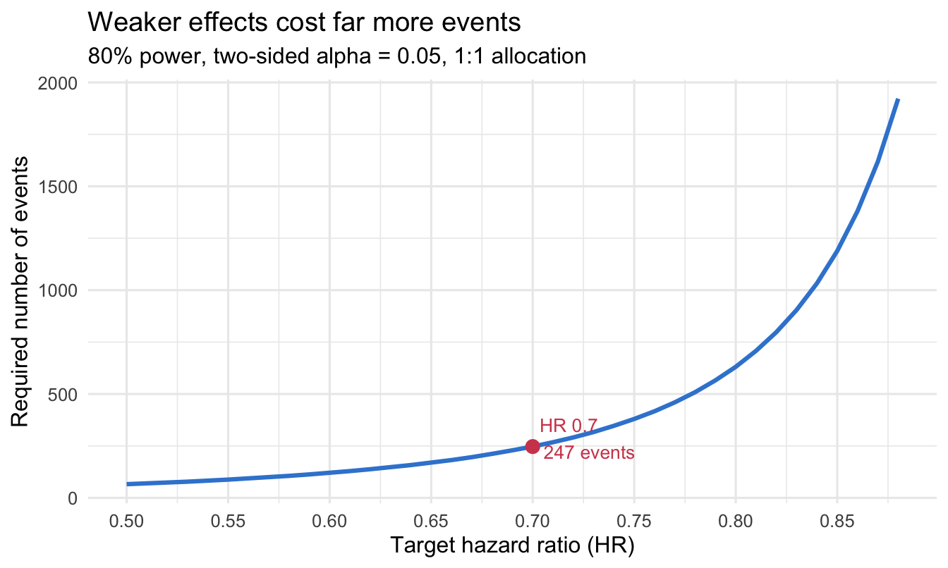
The required events are brutally non-linear in the hazard ratio. As HR moves toward 1 (a smaller effect), (log HR)² shrinks toward zero and the event requirement explodes. Plot it to feel the cliff — required events against the target HR, at the same 80% power / two-sided 5% / 1:1 design:
library(ggplot2)z_alpha <-qnorm(1-0.05/2)z_beta <-qnorm(0.80)p <-0.5events_needed <-function(HR) (z_alpha + z_beta)^2/ (p * (1- p) * (log(HR))^2)hr_grid <-seq(0.50, 0.88, by =0.01)df <-data.frame(HR = hr_grid, events =ceiling(events_needed(hr_grid)))ggplot(df, aes(x = HR, y = events)) +geom_line(color ="#3a86d4", linewidth =1.1) +geom_point(data =data.frame(HR =0.70, events =247),color ="#d1495b", size =3) +annotate("text", x =0.70, y =247, label ="HR 0.7\n247 events",hjust =-0.12, vjust =0.3, size =3.5, color ="#d1495b") +scale_x_continuous(breaks =seq(0.5, 0.85, 0.05)) +labs(x ="Target hazard ratio (HR)",y ="Required number of events",title ="Weaker effects cost far more events",subtitle ="80% power, two-sided alpha = 0.05, 1:1 allocation" ) +theme_minimal(base_size =12)
Read the cliff: HR 0.5 needs ~66 events; HR 0.7 needs 247; HR 0.8 needs 631; HR 0.85 needs ~1,189. A single optimistic step in the assumed HR can multiply your trial’s size. The design lesson: be honest, even conservative, about the effect you expect — over-optimism here is the most common reason a survival trial ends up underpowered.
Step 7 — Stratified and biomarker-stratified design
If a strong prognostic factor (stage, region, a biomarker) splits the population, you can stratify the randomization and the analysis. Two reasons:
Balance and efficiency. Stratified randomization keeps the arms comparable on the factor; a stratified log-rank test or a stratified Cox model then compares treatments within strata and pools the result, removing the factor’s nuisance variation. See Stratified Cox regression.
Biomarker-targeted effects. When the treatment is expected to work mainly in a biomarker-positive subgroup, a biomarker-stratified design pre-specifies that subgroup as the primary analysis population and powers it on its own event count. The all-comers population becomes a key secondary, tested in a pre-specified hierarchy to control the overall error rate.
Stratification factors should be few (2–3), strongly prognostic, and pre-specified — chosen in the protocol, not after looking at the data. Which leads to the most important design principle of all.
The endpoint, the target HR, the analysis population, the censoring rules, the stratification, and the timing of the analysis must be fixed in the protocol before data are seen. Modern regulatory thinking frames this as the estimand — a precise statement of what you are estimating (the population, the endpoint, how intercurrent events like treatment switching are handled, and the summary measure). A clear estimand makes the sample-size assumptions defensible and the result interpretable.
For the censoring conventions, the ADTTE dataset structure, and the ICH E9 / estimand rigor a regulatory submission expects, see CDISC ADTTE & regulatory survival analysis.
A planning checklist
Before you write the sample-size section, you should be able to answer:
Endpoint — what exactly counts as an event, and what is censored?
Estimand — population, endpoint, intercurrent-event handling, summary measure, all pre-specified.
Try it live
Size your own study. Change the target HR, power, allocation, event probability, and dropout — watch the events and patient count move. The sandbox boots on first Run.
🟢 With an AI agent
Ask Prova“how many events and patients do I need to detect a hazard ratio of 0.75 at 90% power with 2:1 randomization, and how does that change if I expect only half my patients to have the event?” — it answers with the base-R Schoenfeld calculation you can run on your own assumptions. The runtime is the judge.Ask Prova →
Common issues
You powered the study on patients instead of events. The most common — and most expensive — survival-design mistake. A headcount-based calculation that ignores the event rate can enroll thousands and still be underpowered if events are rare or follow-up is short. Always size on events first (Schoenfeld), then back out patients from the event probability.
You ignored dropout (and informative censoring). Patients lost to follow-up are censored before they reach the event, so they cost you events directly — and if dropout is related to prognosis it also biases the HR. Inflate enrollment by 1/(1 − dropout), and design follow-up to minimize loss (administrative censoring at the cutoff is fine; lost-to-follow-up is not).
Your target HR was optimistic. Because required events scale with 1/(log HR)², assuming HR = 0.6 when the true effect is 0.75 can quietly triple the events you actually need — leaving the trial underpowered. Choose the minimal clinically important HR, run a sensitivity table across plausible HRs (the curve above), and size for the conservative end.
Frequently asked questions
NoteHow many events do I need for a survival analysis?
Use the Schoenfeld formula: d = (z_{1−α/2} + z_{1−β})² / (p·(1−p)·(log HR)²). For the common case of 80% power, a two-sided 5% level, and 1:1 allocation it simplifies to d ≈ 7.85 / (log HR)². To detect a hazard ratio of 0.7 you need about 247 events; a hazard ratio of 0.8 needs ~631. The number of patients follows from dividing the events by the proportion expected to have the event.
NoteWhy does survival power depend on the number of events, not the sample size?
Because the log-rank and Cox comparisons extract their information from when events happen relative to the arms. A censored patient — event-free at the cutoff — contributes almost nothing; only patients who have the event sharpen the hazard comparison. So a huge cohort with few events is underpowered, while a modest cohort with many events is well-powered. Patients are just the vehicle for generating the events that carry the power.
NoteWhat is an event-driven trial design?
A design where the primary analysis is triggered when a target number of events is reached, not on a fixed calendar date. If events accrue slower than expected you follow patients longer rather than losing power — the event count, not the clock, decides when to analyze. It is the standard for registration-grade survival trials precisely because it guarantees the planned power.
NoteHow do I convert the required number of events into a number of patients?
Divide the required events by the expected event probability over the study: N = d / Pr(event). If you need 247 events and expect 60% of patients to have the event, that’s 247 / 0.60 ≈ 412 patients. Then inflate for dropout — divide by (1 − dropout fraction) — so that enough analyzable patients remain. Longer follow-up raises Pr(event) and is often cheaper than enrolling more people.
NoteDoes a smaller hazard ratio need a bigger study?
Yes — and the cost rises sharply. Required events scale with 1/(log HR)², so as the HR approaches 1 (a weaker effect) the event requirement explodes: HR 0.5 needs ~66 events, HR 0.7 needs 247, HR 0.85 needs nearly 1,200, at 80% power. This is why an optimistic effect assumption is the most common cause of an underpowered survival trial — size for the smallest effect you would still care about.
Test your understanding
ImportantPractice
Run it. In the live cell below, compute the required number of events to detect a hazard ratio of 0.75 at 90% power, two-sided α = 0.05, with 1:1 allocation. Fill the blanks. How many events?
Then convert. If you expect 50% of patients to have the event and a 15% dropout, how many patients must you enroll?
NoteHint
Set HR <- 0.75 and power <- 0.90. For the conversion, divide the events by the event probability (0.50), then divide by (1 - 0.15) for dropout. qnorm(0.90) ≈ 1.28 is the z for 90% power.
You need ≈ 508 events — far more than the 380 events the same HR needed at 80% power, because raising power from 80% to 90% raises z_beta from 0.84 to 1.28. That translates to ~1,016 analyzable patients, or ~1,196 enrolled after allowing for 15% dropout.
TipQuick check
A team plans a trial with 4,000 patients but a 2-year follow-up in a disease where only ~5% of patients have the event in 2 years. Is the study well-powered for a survival comparison?
NoteShow answer
Probably not — too few events. 5% of 4,000 ≈ 200 events, regardless of the large headcount. Whether that’s enough depends on the target HR (200 events covers about HR 0.74 at 80% power), but the point is that the 4,000 patients are irrelevant on their own — only the ~200 events carry the power. Lengthen follow-up or choose an endpoint with a higher event rate to generate more events.
Conclusion
Designing a time-to-event study starts with one shift in thinking: power is driven by events, not patients. Pin down the endpoint, choose the smallest hazard ratio worth detecting, and compute the required events with the Schoenfeld formula — d ≈ 247 for HR 0.7 at 80% power, 1:1 allocation. Convert events to patients through the expected event probability, inflate for dropout, and plan accrual and follow-up long enough to reach the event target — the event-driven trigger then guarantees your power. Be conservative about the effect size, pre-specify any stratification, and frame the whole plan as a clear estimand. Do that, and your sample-size section is both defensible and right.
Every result on this page was produced by the code shown, run at build time against a pinned R environment — edit any block and Run to reproduce it yourself.