Linear Regression Assumptions and Diagnostics in R

After you fit a model, check it. Read the four diagnostic plots, test linearity, normality and homoscedasticity, and find outliers and influential points — with the fixes when an assumption fails

Check the assumptions of a linear regression in R: linearity, normality of residuals, homogeneity of variance (homoscedasticity), and influential observations. Read the four base-R diagnostic plots (residuals vs fitted, normal Q-Q, scale-location, residuals vs leverage), detect outliers, high-leverage and influential points with Cook’s distance — and the workaround for each violation. Run it all live.

TipKey takeaways

• After you fit a regression, always check it. Linear regression assumes linearity, normal residuals, constant residual variance (homoscedasticity), and no influential outliers.
• The four base-R diagnostic plots — plot(model) — check all of them: Residuals vs Fitted (linearity), Normal Q-Q (normality), Scale-Location (homoscedasticity), Residuals vs Leverage (influence).
• Residuals are the gap between observed and fitted values; almost every diagnostic reads the residuals.
• Outliers = extreme outcome values (standardized residual > 3); high-leverage = extreme predictor values (hat value > 2(p+1)/n); influential = changes the fit when removed (Cook’s distance > 4/(n−p−1)).
• Each violation has a fix: transform a predictor (non-linearity), transform the outcome (heteroscedasticity), or investigate/exclude an influential point.

Introduction

Fitting a linear regression is only half the job — a model can return a slope, an R² and a p-value while quietly violating the assumptions those numbers rely on. Regression diagnostics check whether the model actually fits the data, so you can trust the result (or fix it).

Linear regression assumes four things. This lesson shows how to check each one with R’s built-in diagnostic plots, how to read them, and — the practical part — what to do when an assumption fails.

The data and a model to check

We use the marketing dataset from datarium and fit a simple model predicting sales from the youtube advertising budget:

data("marketing", package = "datarium")

model <- lm(sales ~ youtube, data = marketing)
model

Call:
lm(formula = sales ~ youtube, data = marketing)

Coefficients:
(Intercept)      youtube  
    8.43911      0.04754  

The fitted line is sales = 8.44 + 0.0475 × youtube. Now let’s check whether this model is sound.

Fitted values and residuals

Two concepts underlie every diagnostic. The fitted (predicted) value is what the model expects for a given predictor; the residual is the gap between the observed value and that fitted value:

data("marketing", package = "datarium")
model <- lm(sales ~ youtube, data = marketing)

marketing$fitted <- fitted(model)

plot(marketing$youtube, marketing$sales, pch = 19, col = "grey40",
     xlab = "YouTube budget (k$)", ylab = "Sales")
abline(model, col = "#3a86d4", lwd = 2)
segments(marketing$youtube, marketing$sales,
         marketing$youtube, marketing$fitted, col = "red")

Each red segment is a residual error. The diagnostics that follow all examine the distribution of these residuals — if the model is right, the residuals should be patternless, evenly spread, and roughly normal. You can pull them out directly with base R:

data("marketing", package = "datarium")
model <- lm(sales ~ youtube, data = marketing)

diag <- data.frame(
  fitted     = fitted(model),         # predicted sales
  resid      = residuals(model),      # observed - fitted
  std_resid  = rstandard(model),      # standardized residual (outlier check)
  hat        = hatvalues(model),      # leverage (extreme predictor check)
  cooksd     = cooks.distance(model)  # influence (Cook's distance)
)
head(diag, 4)

     fitted    resid std_resid         hat      cooksd
1 21.564929 4.955071 1.2733486 0.009703067 0.007943433
2 10.977569 1.502431 0.3865746 0.012168549 0.000920434
3  9.420269 1.739731 0.4486150 0.016493630 0.001687550
4 17.081273 5.118727 1.3123012 0.005013546 0.004338753

The four diagnostic plots

plot(model) produces the four standard diagnostic plots at once — the fastest way to screen a model:

data("marketing", package = "datarium")
model <- lm(sales ~ youtube, data = marketing)

par(mfrow = c(2, 2))
plot(model)

par(mfrow = c(1, 1))

Read them as four checks:

1. Residuals vs Fitted → linearity. A roughly horizontal red line with no pattern is good.
2. Normal Q-Q → normality of residuals. Points should hug the dashed line.
3. Scale-Location → homoscedasticity (constant variance). A flat line with evenly spread points is good.
4. Residuals vs Leverage → influential points. Watch for points outside the Cook’s-distance contours.

Each plot labels the 3 most extreme observations by row number (#26, #36, #179 here) — worth a look, but not automatically a problem. The next sections take each assumption in turn.

Linearity of the data

Check the Residuals vs Fitted plot (plot 1). Ideally the red line is approximately horizontal at zero — a pattern signals that the straight-line model is wrong:

data("marketing", package = "datarium")
model <- lm(sales ~ youtube, data = marketing)

plot(model, 1)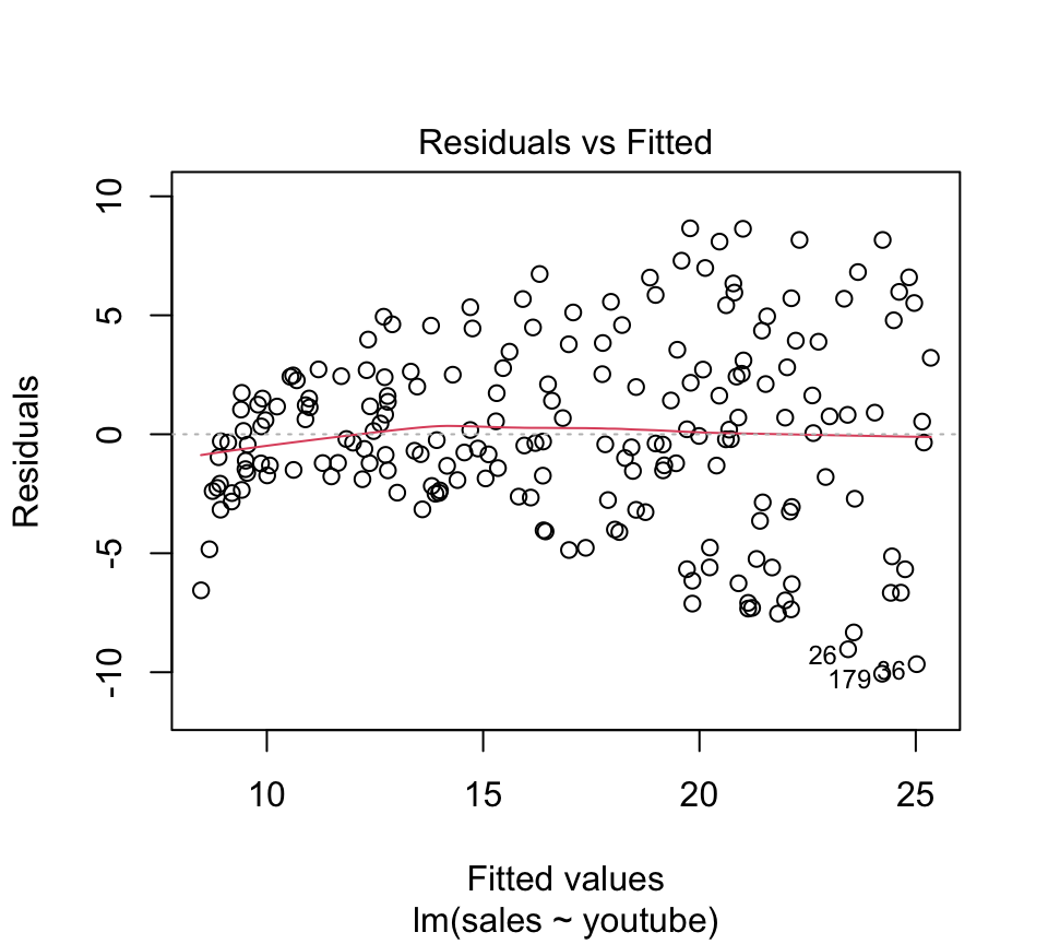

Tip

Verdict here: no strong pattern — the linearity assumption is reasonable. If it failed (a clear curve), the fix is a non-linear transformation of the predictor — log(x), sqrt(x), or a polynomial term poly(x, 2) — then re-check this plot.

Homogeneity of variance (homoscedasticity)

Check the Scale-Location plot (plot 3). A horizontal line with evenly spread points means constant variance; an upward trend means the spread grows with the fitted value — heteroscedasticity:

data("marketing", package = "datarium")
model <- lm(sales ~ youtube, data = marketing)

plot(model, 3)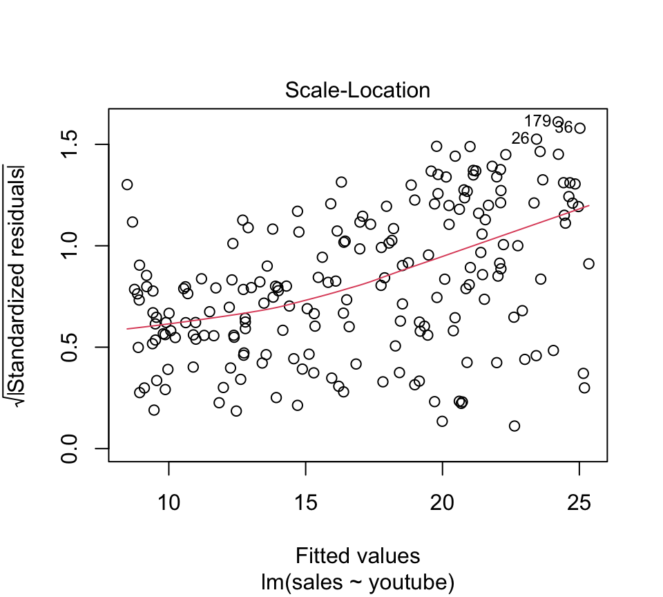

Warning

Verdict here: the line trends up — the residual variance increases with predicted sales, so this model has a heteroscedasticity problem. The fix is a log or square-root transformation of the outcome:

data("marketing", package = "datarium")

model_log <- lm(log(sales) ~ youtube, data = marketing)
plot(model_log, 3)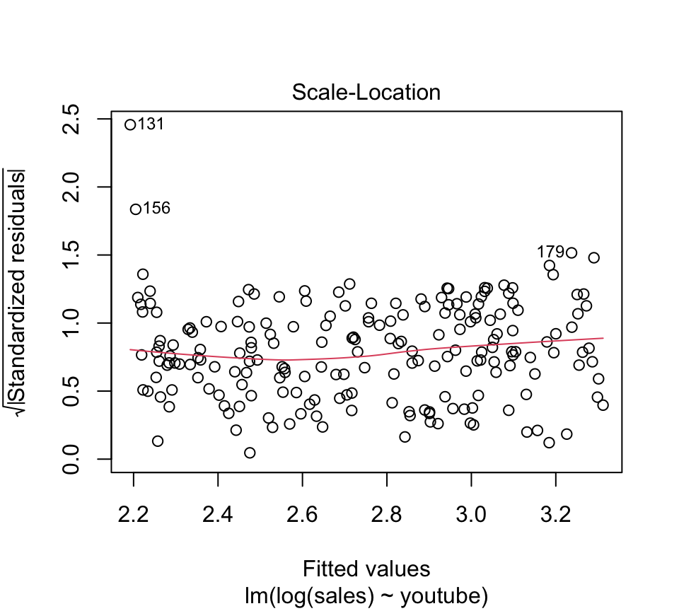

After modelling log(sales), the scale-location line is much flatter — the variance is stabilised.

Normality of residuals

Check the Normal Q-Q plot (plot 2). If the residuals are normal, the points fall along the dashed reference line:

data("marketing", package = "datarium")
model <- lm(sales ~ youtube, data = marketing)

plot(model, 2)

Tip

Verdict here: the points follow the line closely — normality is a safe assumption. With a large sample the F- and t-tests are robust to mild departures anyway; worry only about strong curving or heavy tails. If it failed, a transformation of the outcome often helps (and frequently fixes heteroscedasticity at the same time).

Outliers and high-leverage points

Two different kinds of extreme observation, read off the Residuals vs Leverage plot (plot 5):

• An outlier has an extreme outcome value — detected by the standardized residual. A value beyond ±3 is a possible outlier.
• A high-leverage point has an extreme predictor value — detected by the hat value. A value above 2(p + 1)/n is high leverage (p = number of predictors, n = observations).

data("marketing", package = "datarium")
model <- lm(sales ~ youtube, data = marketing)

plot(model, 5)

Tip

Verdict here: the three labelled points (#26, #36, #179) have standardized residuals between −2 and −3 — extreme but none beyond ±3, so no genuine outliers. And every hat value is below 2(p + 1)/n = 4/200 = 0.02, so there are no high-leverage points either.

Influential values (Cook’s distance)

An influential point is one whose inclusion or exclusion would change the regression result. It combines leverage and residual size, measured by Cook’s distance — flagged when it exceeds 4/(n − p − 1). Plot Cook’s distance and Residuals vs Leverage side by side:

data("marketing", package = "datarium")
model <- lm(sales ~ youtube, data = marketing)

par(mfrow = c(1, 2))
plot(model, 4)   # Cook's distance
plot(model, 5)   # Residuals vs Leverage

par(mfrow = c(1, 1))

Inspect the highest-Cook’s-distance rows directly with base R:

data("marketing", package = "datarium")
model <- lm(sales ~ youtube, data = marketing)

cd <- cooks.distance(model)
marketing[order(cd, decreasing = TRUE)[1:3], ]   # top 3 most influential rows

    youtube facebook newspaper sales
36   348.84     4.92     10.20 15.36
179  332.04     2.76     28.44 14.16
26   315.48     4.20     23.40 14.40

Tip

Verdict here: no influential points. The Cook’s-distance contour lines don’t even appear on the Residuals-vs-Leverage plot because every point sits comfortably inside them — excluding any single observation would barely move the fit.

What an influential point looks like

To see the contrast, add two extreme points and refit — now the diagnostics light up:

data("marketing", package = "datarium")

df2 <- data.frame(
  x = c(marketing$youtube, 500, 600),
  y = c(marketing$sales, 80, 100)
)
model2 <- lm(y ~ x, data = df2)

par(mfrow = c(1, 2))
plot(model2, 4)
plot(model2, 5)

par(mfrow = c(1, 1))

Observations #201 and #202 sit far beyond the Cook’s-distance lines — they are influential. Excluding them shifts the slope (here from ~0.065 back toward ~0.048). When a point is both high-Cook’s-distance and at the edge of the leverage plot, decide deliberately: is it a data-entry error (fix or drop it) or a real, important observation (keep it, and report the sensitivity)?

Diagnosis summary

Assumption	Plot	Good sign	Fix if violated
Linearity	Residuals vs Fitted	flat red line	transform predictor: log(x), poly(x, 2)
Normality	Normal Q-Q	points on the line	transform outcome; large-n is robust
Homoscedasticity	Scale-Location	flat, even spread	transform outcome: log(y), sqrt(y)
No influence	Residuals vs Leverage + Cook’s	inside the contours	investigate / exclude the point

NoteThe math (optional)

The standardized residual is \(r_i = \dfrac{e_i}{s\sqrt{1 - h_i}}\), where \(e_i\) is the raw residual, \(s\) the residual standard error, and \(h_i\) the leverage (hat value). Leverage \(h_i\) is the \(i\)-th diagonal of the hat matrix \(H = X(X^\top X)^{-1}X^\top\), with \(\sum_i h_i = p + 1\) — hence the 2(p+1)/n rule (twice the average). Cook’s distance combines residual and leverage, \(D_i = \dfrac{r_i^2}{p + 1}\cdot\dfrac{h_i}{1 - h_i}\) — large when a point is both far from the line and extreme in the predictors.

Try it live

Refit with the log of sales and re-run the diagnostics — does the scale-location plot flatten out? The sandbox boots on first Run.

🟢 With an AI agent

Ask Prova “check the assumptions of my regression and tell me which one is violated and how to fix it” — it reads your diagnostic plots and answers with code you can run on your own model. The runtime is the judge. Ask Prova →

Common issues

You treated a labelled point as an automatic outlier. plot(model) labels the 3 most extreme rows by default — that’s just “look here,” not “remove these.” Check the actual cut-offs: standardized residual > 3 (outlier), hat > 2(p+1)/n (leverage), Cook’s distance > 4/(n−p−1) (influence).

You saw a pattern in residuals and panicked. A pattern isn’t a stop signal — it’s information. A curve in Residuals-vs-Fitted suggests a transformation or a missing term; a funnel in Scale-Location suggests a log/sqrt outcome. Fix the model, don’t abandon it.

Heteroscedasticity with a valid model. If a transformation isn’t desirable, keep the model but use robust (heteroscedasticity-consistent) standard errors for inference (e.g. sandwich + lmtest), so the p-values and CIs stay valid.

Frequently asked questions

NoteWhat are the assumptions of linear regression?

Four: linearity (the predictor–outcome relationship is a straight line), independence of the residual errors, normality of the residuals, and homoscedasticity (constant residual variance). You also check for influential observations that distort the fit. All are diagnosed by examining the residuals.

NoteHow do I check regression assumptions in R?

Fit the model with lm(), then call plot(model) for the four diagnostic plots: Residuals vs Fitted (linearity), Normal Q-Q (normality), Scale-Location (homoscedasticity), and Residuals vs Leverage (influential points). Read each plot against its assumption; back them with rstandard(), hatvalues() and cooks.distance().

NoteHow do I detect outliers and influential points in regression?

An outlier has a standardized residual (rstandard()) beyond ±3. A high-leverage point has a hat value (hatvalues()) above 2(p+1)/n. An influential point has a Cook’s distance (cooks.distance()) above 4/(n−p−1) — it’s the one that actually changes the fit when removed. The Residuals-vs-Leverage plot shows all three at once.

NoteWhat do I do if an assumption is violated?

It depends which: non-linearity → transform the predictor (log, sqrt, poly); heteroscedasticity → transform the outcome (log(y), sqrt(y)) or use robust standard errors; non-normal residuals → transform the outcome (large samples are fairly robust); an influential point → investigate it (data error vs real) and report the analysis with and without it.

Test your understanding

ImportantPractice

1. Run it. In the live cell, compare the Scale-Location plot of lm(sales ~ youtube) with lm(log(sales) ~ youtube). Which one shows constant variance?
2. Conceptual. A point has a large standardized residual but a low hat value. Is it likely to be influential (change the fit)? Why or why not?

NoteHint

Fill the blank with sales, then log(sales), and watch the red line in the scale-location plot. For question 2, recall that Cook’s distance combines both residual size and leverage.

NoteSolution

plot(lm(sales ~ youtube, data = marketing), 3)        # line trends up: heteroscedastic
plot(lm(log(sales) ~ youtube, data = marketing), 3)   # much flatter: variance stabilised

The log(sales) model has the more constant variance. For question 2: probably not influential. Cook’s distance multiplies residual size by leverage; a large residual at low leverage (a typical predictor value) gets little weight, so removing the point barely moves the line. Influence needs both an unusual outcome and an unusual predictor value.

Conclusion

You can now diagnose a linear regression in R: read the four plot(model) diagnostics, check linearity (Residuals vs Fitted), normality (Q-Q), homoscedasticity (Scale-Location), and influence (Residuals vs Leverage + Cook’s distance) — and apply the right fix for each violation, from transforming a variable to handling an influential point. A model you’ve checked is a model you can report.

Related lessons

• Simple linear regression in R · Multiple linear regression in R — fit the models you diagnose here. · Multicollinearity & VIF in R — the extra assumption for multiple regression. · Logistic regression assumptions & diagnostics in R — the equivalent checks for a binary outcome.
• Go further: Regression analysis · Biostatistics

Was this page helpful?

Prove you can do it. Master the whole Regression in R series — track your path, build projects, and earn a certificate.

Start free →

Go Pro — unlimited Prova on your own data and a verifiable certificate that proves the skill.

from $15/mo billed yearly

Go Pro →

✓ You're Pro — keep going. The runtime is the judge.

Ready to level up?

Try this on your own data with Prova — the runtime is the judge.Open Prova →

Get new R & Python lessons by email

Practical, reproducible, no spam. Unsubscribe anytime.

Double opt-in. We never share your email.

Share this pageXLinkedInRedditHN

Note

Every result on this page was produced by the code shown, run at build time against a pinned R environment — edit any block and Run to reproduce it yourself.