ADTTE Analysis Example in R: A Complete Regulatory Survival Package
The end-to-end deliverable a biostatistician produces for a clinical study report — the primary time-to-event analysis on a CDISC ADTTE dataset (KM, stratified log-rank, the Cox hazard ratio, CSR tables and figure) plus the sensitivity analysis set that defends it: RMST, competing risks, and a subgroup check, framed by ICH E9(R1)
Biostatistics
A complete, worked regulatory time-to-event analysis package on a CDISC ADTTE dataset in R. Build the analysis-ready Surv() object from the CNSR flag, run the pre-specified PRIMARY analysis (Kaplan-Meier with median and 95% CI, stratified log-rank, the primary Cox hazard ratio with a proportional-hazards check, the submission figure and gtsummary CSR tables), then add the SENSITIVITY analysis set that makes it defensible — restricted mean survival time (survRM2) as a PH-free effect, a competing-risks cumulative-incidence view (tidycmprsk), and a subgroup / stratified consistency check. Assemble the submission outputs and write the regulatory report paragraph with ICH E9(R1) estimand framing.
Published
June 26, 2026
Modified
July 7, 2026
TipKey takeaways
A regulatory time-to-event deliverable is not one number — it is a pre-specified primary analysis plus a sensitivity set that shows the result holds when you change the method. This capstone builds the whole package on one CDISC ADTTE dataset.
Primary analysis (the pre-specified estimand): Kaplan-Meier with median OS + 95% CI, the stratified log-rank test, the Cox hazard ratio with a PH check, plus the submission figure and gtsummary CSR tables. On the ADTTE-shaped colon-cancer trial, Lev+5FU cut the hazard of death by ~30% (HR = 0.70, 95% CI 0.55–0.88, p = 0.003), proportional hazards holding (p = 0.34).
Sensitivity analysis (the value-add that defends the primary): RMST (a PH-free, interpretable effect — +111 days over 5 years, p = 0.020); a competing-risks cumulative-incidence view (death vs the competing event of recurrence); and a subgroup / stratified consistency check (HR 0.68 in patients with <4 nodes, 0.72 in 4+; interaction p = 0.92).
The point of a sensitivity set is convergence: if the absolute (RMST), the assumption-free, and the subgroup analyses all point the same way as the primary HR, the conclusion is robust. If one diverges, you have found something — and you report it.
Frame the whole package with ICH E9(R1): a pre-specified estimand, documented censoring rules, named stratification factors, and primary-vs-sensitivity roles fixed in the SAP before unblinding.
Introduction
You have the CDISC ADTTE mapping down — you can take a time-to-event endpoint from an ADaM dataset to a correct Surv() object and fit the primary model. This capstone is the next step: the complete analysis package a biostatistician hands over for a clinical study report.
A real submission is never a lone hazard ratio. It is a pre-specified primary analysis that defines the treatment effect, wrapped in a sensitivity analysis set whose only job is to ask “would a reviewer who distrusted my method reach the same conclusion?” Change the summary measure, drop the proportional-hazards assumption, account for a competing event, look within subgroups — if the answer stays the same, the result is robust. That convergence is what makes a finding defensible, and assembling it is the work this lesson walks through end to end.
We build it on one ADTTE dataset and run, in order:
the primary analysis — KM + median/CI, stratified log-rank, the Cox HR, the PH check, the submission figure and the CSR tables;
the sensitivity set — RMST (a PH-free, interpretable effect), a competing-risks cumulative-incidence view, and a subgroup consistency check;
the assembly — the submission outputs and the ICH E9(R1)-framed report.
This is the project that applies everything in the series. If you want the mechanics of any one step explained from scratch, the cross-links point to the lesson that teaches it; here we put them together the way the work actually happens.
The ADTTE dataset (built once, used throughout)
Real ADTTE data is confidential, so we derive a CDISC-shaped ADTTE dataset from the public colon trial that ships with survival — an adjuvant therapy trial in colon cancer. The CDISC ADTTE lesson explains every variable and the mapping in detail; here we build it once and move on. Two things carry the whole analysis:
The censoring flip. CDISC codes CNSR = 1 as censored (the opposite of R’s Surv(time, event), which wants event = 1). We map raw colon$status (1 = death) to CNSR = 1 - status, then rebuild the R event indicator as event = 1 - CNSR. Get this backwards and every result is silently wrong.
One row per subject per parameter. We take the death records (etype == 2) as the overall-survival parameter and two arms — Observation vs Lev+5FU.
library(survival)# Overall-survival records (death endpoint), two armsos <-subset(colon, etype ==2& rx %in%c("Obs", "Lev+5FU"))os$rx <-droplevels(os$rx)# Map raw trial data to a CDISC ADaM ADTTE structureadtte <-data.frame(USUBJID =sprintf("COLON-ADJ-001-%04d", os$id),PARAMCD ="OS",AVAL = os$time, # time to event / censoring (days)CNSR =1- os$status, # CDISC: 1 = censored, 0 = eventTRT01P =factor(os$rx, levels =c("Obs", "Lev+5FU"),labels =c("Observation", "Lev+5FU")),STRAT =factor(ifelse(os$differ ==3, "Poor", "Well/Moderate")), # stratification factorNODE4 =factor(ifelse(os$node4 ==1, "4+ positive nodes", "<4 positive nodes")), # subgroupstringsAsFactors =FALSE)adtte <- adtte[!is.na(adtte$STRAT), ] # drop unknown stratum# Rebuild the R event indicator from the CDISC censoring flag — the load-bearing lineadtte$event <-1- adtte$CNSR# Sanity check: events must equal CNSR == 0cat("Subjects:", nrow(adtte)," | Events (deaths):", sum(adtte$event)," | Censored (CNSR == 1):", sum(adtte$CNSR ==1), "\n")
606 subjects (308 Observation, 298 Lev+5FU), 287 deaths, the rest censored — alive at last follow-up. The event count matches sum(CNSR == 0), so the censoring flip is right. This adtte is the one dataset the primary and sensitivity analyses below all run on.
Part 1 — the primary analysis (the pre-specified estimand)
The primary analysis estimates the pre-specified effect: overall survival, compared between arms, summarised by the hazard ratio, with the stratified log-rank as the matching test. Everything here is fixed in the SAP before unblinding.
Call: survfit(formula = Surv(AVAL, event) ~ TRT01P, data = adtte)

                     n events median 0.95LCL 0.95UCL
TRT01P=Observation 308    165   2083    1548    2789
TRT01P=Lev+5FU     298    122     NA    2725      NA
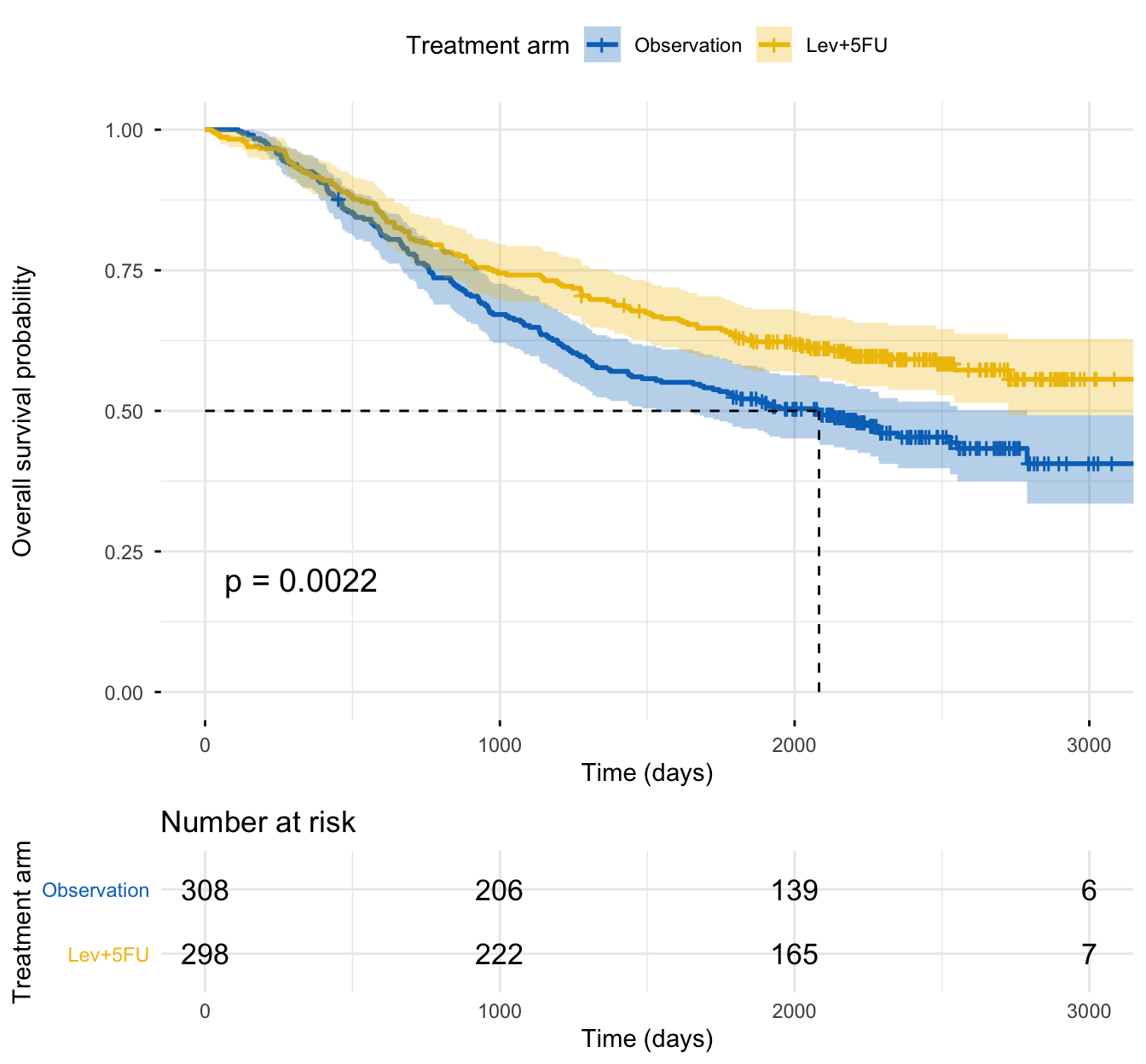
Observation: median OS = 2083 days (95% CI 1548–2789).
Lev+5FU: median = NA (“not reached”) — fewer than half the treated subjects died within follow-up, so the curve never crosses 0.5. That is a good sign, not missing data: report the lower CI bound (2725 days) and a fixed-time survival probability instead.
The submission figure
The Kaplan-Meier plot with a risk table, confidence bands, median lines, and the log-rank p is the standard survival figure in a CSR. Draw it with survminer’s ggsurvplot():
library(survival)library(survminer)os <-subset(colon, etype ==2& rx %in%c("Obs", "Lev+5FU"))os$rx <-droplevels(os$rx)adtte <-data.frame(AVAL = os$time, CNSR =1- os$status,TRT01P =factor(os$rx, levels =c("Obs", "Lev+5FU"),labels =c("Observation", "Lev+5FU")),STRAT =factor(ifelse(os$differ ==3, "Poor", "Well/Moderate")))adtte <- adtte[!is.na(adtte$STRAT), ]adtte$event <-1- adtte$CNSRfit <-survfit(Surv(AVAL, event) ~ TRT01P, data = adtte)ggsurvplot( fit, data = adtte,risk.table =TRUE, # number at risk under the plot (a submission requirement)conf.int =TRUE, # 95% confidence bandspval =TRUE, # log-rank p-value on the plotsurv.median.line ="hv", # dashed median-survival guidespalette ="jco", # colourblind-safe journal palettelegend.labs =c("Observation", "Lev+5FU"),legend.title ="Treatment arm",xlab ="Time (days)",ylab ="Overall survival probability",ggtheme =theme_minimal())
The Lev+5FU curve sits above Observation at every time point — a consistent advantage, curves clearly separated and not crossing.
Stratified log-rank and the primary Cox hazard ratio
The protocol pre-specifies stratifying by tumour differentiation, so the test and the model both stratify on it. The stratified log-rank answers “do the arms differ within strata?”; the stratified Cox gives the effect size — the hazard ratio, the primary estimand.
Stratified log-rank: χ² = 9.1 on 1 df, p = 0.003 — the arms differ within differentiation strata.
HR = 0.70 (95% CI 0.55–0.88) — Lev+5FU multiplies the hazard of death by 0.70, a 30% lower hazard ((1 − 0.70) × 100). Observation is the reference, so the HR reads “treated vs control”.
CI entirely below 1 and the Wald p = 0.003 — convincing; no plausible value where treatment is harmful or null.
This is the headline number the rest of the package has to survive.
Check the proportional-hazards assumption
A single hazard ratio is only meaningful if the effect is constant over time. Check it with cox.zph() (Schoenfeld residuals) before you trust the HR as a summary:
       chisq df    p
TRT01P 0.912  1 0.34
GLOBAL 0.912  1 0.34
χ² = 0.91, p = 0.34 — no evidence the hazard ratio changes over time. The single HR is a valid summary. (When this test is significant, the constant HR misleads — see testing the PH assumption — and the RMST sensitivity below becomes the primary defence.)
The CSR tables — gtsummary
A clinical study report presents clean tables, not raw R output. gtsummary turns the same fitted objects into submission-style tables. First the fixed-time survival probability per arm:
At 5 years, 52% of the Observation arm versus 63% of Lev+5FU are still alive — the advantage as a fixed-time estimate (useful precisely because the treated median was “not reached”). Then the primary estimand as a tbl_regression:
Abbreviations: CI = Confidence Interval, HR = Hazard Ratio
exponentiate = TRUE reports hazard ratios with the 95% CI and p — the exact row for the CSR efficacy table: HR 0.70 (95% CI 0.55, 0.88), p = 0.003, Observation as reference. That is the primary analysis, complete. Now we defend it.
Part 2 — the sensitivity analysis set (the value-add)
A reviewer’s job is to find the assumption that, if wrong, breaks your conclusion. A sensitivity analysis re-runs the comparison under a different assumption or summary measure. The deliverable is not three more p-values — it is a statement about robustness: do the alternative analyses converge with the primary HR, or does one diverge and tell you something the HR hid?
NotePrimary vs sensitivity — the roles, fixed in advance
Primary analysis — the one pre-specified estimate the trial’s conclusion rests on (here the stratified Cox HR). It defines the estimand and is fixed in the SAP before unblinding.
Sensitivity analyses — pre-specified alternatives that stress a specific assumption of the primary: a different summary measure (RMST, no PH assumption), a different event structure (competing risks), a different population slice (subgroups). They support or qualify the primary; they do not replace it, and you do not pick the one with the smallest p after the fact.
Sensitivity (a) — RMST, a PH-free interpretable effect
The hazard ratio assumes proportional hazards and reports a relative effect. Restricted mean survival time assumes neither: it is the area under the survival curve up to a horizon τ — the average survival time within the first τ units — so the effect is an absolute number of days, valid even if PH fails. Run it at a pre-specified 5-year horizon with survRM2::rmst2() (the arm coded 0/1):
RMST difference = 111 days (95% CI 18–204), p = 0.020. Over 5 years, treated patients live on average about 111 days — roughly 3.7 months — longer (RMST ratio 1.08). This converges with the primary HR: a different, assumption-free summary measure points the same way, and now the benefit is expressed as time a patient understands. Because the PH check passed, RMST here is a confirmatory sensitivity; had PH failed, it would have been the analysis you led with.
Sensitivity (b) — a competing-risks view
The OS analysis treats every non-death as censoring. But in this trial a patient can also have cancer recurrence before dying, and death without recurrence is a competing event for recurrence: a patient who dies first can never be observed to recur. Reading recurrence risk off a naive 1 − KM curve would overstate it. The honest summary is the cumulative incidence function (CIF), which accounts for the competing event. Build the competing-risks event variable (a factor with the censor level first) and estimate the CIF by arm with tidycmprsk::cuminc():
library(survival)library(tidycmprsk)# Per subject, merge the recurrence (etype==1) and death (etype==2) recordsco <-subset(colon, rx %in%c("Obs", "Lev+5FU"))rec <- co[co$etype ==1, c("id", "time", "status", "rx", "differ")]dth <- co[co$etype ==2, c("id", "time", "status")]names(rec) <-c("id", "rtime", "rstat", "rx", "differ")names(dth) <-c("id", "dtime", "dstat")cr <-merge(rec, dth, by ="id")# One event time and one competing-risks event codecr$etime <-pmin(cr$rtime, cr$dtime)ecode <-with(cr, ifelse(rstat ==1, 1, ifelse(dstat ==1, 2, 0))) # 1 = recurrence, 2 = deathcr$event <-factor(ecode, levels =c(0, 1, 2),labels =c("censor", "recurrence", "death")) # censor level FIRSTcr$TRT01P <-factor(cr$rx, levels =c("Obs", "Lev+5FU"),labels =c("Observation", "Lev+5FU"))table(cr$event)
    censor recurrence      death
       295        296         28
So 296 recurrences, 28 deaths without recurrence (the competing event), and 295 censored. Now the CIF of recurrence by arm, with Gray’s test:
Recurrence CIF at 5 years: 55% (Observation) vs 38% (Lev+5FU); Gray’s test p < 0.001. The treatment strongly reduces the cumulative incidence of recurrence, accounting for the competing risk of death — a large, significant benefit on the recurrence endpoint.
Death (competing event): Gray’s p = 0.70 — the two arms’ competing mortality is similar, so the recurrence comparison is not distorted by differential competing risk.
This is exactly what a sensitivity analysis should do: it converges in direction with the OS benefit and adds evidence the OS analysis can’t — that the drug’s effect shows up clearly on disease recurrence too, correctly accounted for competing mortality.
Sensitivity (c) — a subgroup / stratified consistency check
The last sensitivity asks whether the primary effect is consistent across the population or driven by one slice. Estimate the HR within a clinically meaningful subgroup (number of positive lymph nodes, a strong prognostic factor) and test the treatment × subgroup interaction — a significant interaction would mean the effect differs by subgroup:
<4 positive nodes: HR = 0.68 (95% CI 0.50–0.91, p = 0.011); 4+ nodes: HR = 0.72 (95% CI 0.50–1.05, p = 0.086). The point estimates are nearly identical; the wider CI in the smaller, higher-risk 4+ group is a power issue, not a different effect.
Interaction p = 0.92 — no evidence the treatment effect differs by nodal status. The benefit is consistent across subgroups.
Three sensitivities, all converging on the primary: an absolute PH-free effect (RMST), an assumption-free competing-risks view, and a consistent subgroup effect. The conclusion is robust.
TipThe sensitivity set at a glance
Analysis
Question it stresses
Result
Verdict
Primary — stratified Cox
The pre-specified relative effect
HR 0.70 (0.55–0.88), p = 0.003
Benefit
RMST (τ = 5 yr)
Drop the PH assumption; absolute effect
+111 days (18–204), p = 0.020
Converges
Competing risks (recurrence CIF)
Account for the competing event
38% vs 55% at 5 yr, Gray’s p < 0.001
Converges
Subgroup (nodal status)
Consistency across the population
HR 0.68 vs 0.72, interaction p = 0.92
Consistent
Assemble the package — the regulatory report
The deliverable pulls the primary and the sensitivities into one paragraph that states the estimand, the primary result, and the consistency of the sensitivity set:
Overall survival was analysed on the Full Analysis Set from the ADTTE dataset (PARAMCD = OS; n = 606, 287 deaths), comparing Lev+5FU with observation. The pre-specified primary analysis — a stratified Cox model (stratification factor: tumour differentiation) — gave a hazard ratio of 0.70 (95% CI 0.55–0.88) in favour of Lev+5FU (stratified log-rank p = 0.003); the proportional-hazards assumption was satisfied (p = 0.34). Median overall survival was 2083 days (95% CI 1548–2789) under observation and was not reached under Lev+5FU; 5-year survival was 52% versus 63%. Pre-specified sensitivity analyses were consistent with the primary result: the restricted mean survival time over a 5-year horizon favoured treatment by 111 days (95% CI 18–204, p = 0.020); the cumulative incidence of cancer recurrence, accounting for the competing risk of death, was lower under treatment (38% vs 55% at 5 years, Gray’s p < 0.001) with similar competing mortality between arms (p = 0.70); and the treatment effect was consistent across nodal subgroups (HR 0.68 for <4 nodes, 0.72 for 4+; interaction p = 0.92). The estimand, analysis population, censoring rules, stratification factor, and the primary-versus-sensitivity roles were defined in the statistical analysis plan, per ICH E9(R1), before unblinding.
NoteICH E9(R1) — what makes this package “submission-grade”
The statistics above are only regulatory if a few things were settled before the analysis. You don’t need a compliance manual — you need to honour what was pre-specified:
A defined estimand. Population (the FAS/ITT), endpoint (PARAMCD = OS, time from randomisation to death from any cause), treatment condition (TRT01P), intercurrent-event strategy, and summary measure (the hazard ratio). The HR is reported for that estimand, not as a generic association.
Primary vs sensitivity roles, fixed in advance. The primary estimate and each sensitivity (RMST, competing risks, subgroup) are pre-specified in the SAP — you do not promote a sensitivity to primary, or cherry-pick the τ / subgroup / method with the smallest p, after seeing the data.
Documented censoring rules.CNSR, EVNTDESC, and CNSDTDESC make every subject’s status auditable — event or censoring, on what date and why.
Named stratification factors enter the stratified log-rank and Cox, so the treatment effect is estimated within prognostic strata.
Traceability. Every number traces SDTM → ADaM (ADTTE) → analysis output, reproducibly.
NoteWhen this package has to be audited and validated — Arkon
Everything on this page is the statistics of a regulatory analysis package — the primary estimand and a defensible sensitivity set, reproducibly. Turning it into an actual submission deliverable adds a production layer: double-programmed analyses validated against the SAP, full SDTM → ADaM → TLF traceability, version control, and a documented audit trail a regulator can follow end to end. That production discipline — reproducible, validated, agent-assisted clinical-analysis pipelines — is what Arkon is built for. Use this lesson to build the analysis package; reach for Arkon when it has to be audited and validated for a real filing.
Common issues
You promoted a sensitivity analysis to primary because its p was smaller. The primary analysis is fixed in the SAP before unblinding; a sensitivity that happens to be more significant does not become the headline. Report the pre-specified primary as the conclusion and the sensitivities as support. Swapping roles post hoc is the most common — and most penalised — sensitivity-analysis error.
Your competing-risks event factor wasn’t built correctly.cuminc() and crr() need the event as a factor whose first level is the censoring code. A numeric event, or a factor with the censor level not first, fails or returns nonsense. Build factor(code, levels = c(0, 1, 2), labels = c("censor", ...)) explicitly, and confirm the counts with table().
You read recurrence risk off 1 − KM instead of the CIF. With a real competing event (death before recurrence), the Kaplan-Meier complement overstates the cumulative incidence — it credits patients who died with a future chance to recur. Use cuminc() for any endpoint that has a competing event; reserve 1 − KM for overall survival, where death is the event.
You set the RMST horizon τ after seeing the result. τ defines the estimand and changes the answer (the RMST lesson shows the same data giving p = 0.02 at 5 years and p = 0.18 at 3). Pre-specify τ from the clinical question; reporting the τ that minimises p is fishing.
Frequently asked questions
NoteWhat goes in a regulatory survival analysis?
A submission-grade time-to-event analysis is a package, not one statistic: a pre-specified primary analysis (usually Kaplan-Meier with median and 95% CI, the stratified log-rank test, and the Cox hazard ratio with a proportional-hazards check), the submission outputs (the KM figure with a risk table and CSR-style tables, e.g. via gtsummary), and a sensitivity analysis set that shows the result is robust (commonly RMST, a competing-risks view, and subgroup consistency). It is wrapped in ICH E9(R1) estimand framing — defined population, endpoint, censoring rules, stratification factors — all fixed in the SAP before unblinding.
NoteWhat is the difference between a primary and a sensitivity analysis in survival?
The primary analysis is the single pre-specified estimate the trial’s conclusion rests on (e.g. the stratified Cox hazard ratio); it defines the estimand and is fixed before unblinding. A sensitivity analysis re-runs the comparison under a different assumption or summary measure — RMST (no proportional-hazards assumption), competing risks (a different event structure), subgroups (a different population slice) — to test whether the primary conclusion holds. Sensitivities support or qualify the primary; they never replace it, and you do not promote the one with the smallest p after seeing the data.
NoteWhy include RMST and competing risks as sensitivity analyses?
Each stresses a specific assumption of the primary Cox HR. RMST drops the proportional-hazards assumption and reports an absolute effect (days/months gained), so it is valid even if PH fails and is interpretable for clinicians and patients. Competing risks account for an event (often death) that prevents the event of interest, which a naive 1 − Kaplan-Meier analysis ignores — so the cumulative incidence is estimated honestly. If both converge with the primary HR, the conclusion is robust; if one diverges, it has revealed something the single HR hid.
NoteHow do I interpret a treatment-by-subgroup interaction test?
The interaction p-value asks whether the treatment effect differs across the subgroup. A largep (here 0.92) means no evidence the effect differs — the benefit is consistent, and the per-subgroup hazard ratios (0.68 and 0.72) differ only by chance. A small interaction p would suggest a genuine effect modification worth investigating. Subgroup analyses are sensitivity/consistency checks: read the interaction test, not just the per-subgroup p-values, which are individually underpowered.
NoteIs a CDISC ADTTE dataset required to run this analysis?
No — the survival statistics are the same on any time-to-event data. ADTTE is the CDISC ADaM standard that makes the analysis submission-ready: one record per subject per parameter, fixed variable names (AVAL, CNSR, TRT01P), and documented censoring — so a reviewer can re-run it and get your numbers. For the mapping from ADTTE to Surv() (and the CNSR = 1 censoring flip), see the CDISC ADTTE lesson; this capstone applies that mapping and adds the full primary and sensitivity analysis set.
Test your understanding
ImportantPractice
Assemble it. You have an ADTTE OS endpoint with a significant primary Cox HR of 0.75 and a passing PH check. Name three pre-specified sensitivity analyses you would add, and state the specific assumption each one stresses. What single result across the set would make you least confident in the primary?
Run a sensitivity. Below, compute the RMST sensitivity at a 5-year horizon on the ADTTE data and confirm it converges with the primary HR. Fill the blank with the horizon in days.
TipHint
For (1): the three you built here are RMST (drops the PH assumption / absolute effect), competing risks (accounts for a competing event), and subgroups (consistency across the population). The least-reassuring outcome is a sensitivity that diverges in direction from the primary. For (2): a 5-year horizon is 1825 days; read the first row of res$unadjusted.result — Est. is the RMST difference in days and the last column is its p.
TipSolution
library(survival)library(survRM2)# Build the ADTTE OS data (death records), event = 1 - CNSR, arm coded 0/1os <-subset(colon, etype ==2& rx %in%c("Obs", "Lev+5FU"))os$rx <-droplevels(os$rx)adtte <-data.frame(AVAL = os$time, CNSR =1- os$status,TRT01P =factor(os$rx, levels =c("Obs", "Lev+5FU"),labels =c("Observation", "Lev+5FU")))adtte$event <-1- adtte$CNSRarm <-ifelse(adtte$TRT01P =="Lev+5FU", 1, 0)# RMST sensitivity at the prespecified 5-year horizonres <-rmst2(adtte$AVAL, adtte$event, arm, tau =1825)res$unadjusted.result#> RMST (arm=1)-(arm=0) Est. = 111 days, 95% CI 18-204, p = 0.020 — CONVERGES with HR 0.70.
For question 1: add RMST (stresses the proportional-hazards assumption and gives an absolute effect), a competing-risks cumulative-incidence analysis (stresses the assumption that competing events are just censoring), and a subgroup / interaction analysis (stresses consistency across the population). You would be least confident in the primary if one of these diverged in direction — e.g. an RMST difference near zero or a competing-risks CIF showing no benefit — because that signals the single HR is sensitive to an assumption it depends on. Convergence across the set is what makes the primary defensible.
For question 2: the RMST difference is 111 days (95% CI 18–204, p = 0.020) in favour of treatment — it converges with the primary HR of 0.70, confirming the benefit under a PH-free, absolute summary.
TipQuick check
In your analysis package, a pre-specified sensitivity RMST analysis returns a smaller p-value than the primary Cox model. Should you report the RMST result as the primary conclusion?
NoteShow answer
No. The primary analysis is fixed in the SAP before unblinding; a sensitivity analysis that happens to be more significant does not become the headline. Report the pre-specified primary (the Cox HR) as the conclusion and the RMST as supporting evidence of robustness. Promoting a sensitivity to primary after seeing the results inflates the type-I error rate and is a serious — and penalised — regulatory error. The sensitivity’s value is that it converges with the primary, not that it can replace it.
Conclusion
A regulatory time-to-event deliverable is a package: a pre-specified primary analysis that defines the estimand, plus a sensitivity set that proves it robust. On the CDISC-shaped colon-cancer trial, the primary stratified Cox model gave HR = 0.70 (95% CI 0.55–0.88, p = 0.003) with proportional hazards holding, the submission figure and gtsummary CSR tables alongside. The sensitivity set converged: RMST showed +111 days over 5 years (p = 0.020) as an absolute, PH-free effect; the competing-risks view showed a lower cumulative incidence of recurrence under treatment (Gray’s p < 0.001) once the competing risk of death was accounted for; and the effect was consistent across nodal subgroups (interaction p = 0.92). That convergence — the same conclusion under a different summary, a different event structure, and a different population slice — is what makes the result defensible. Wrap it in ICH E9(R1) estimand framing, fix the primary-versus-sensitivity roles in the SAP before unblinding, and you have the analysis package a clinical study report needs.
Ask Prova“build a complete regulatory survival analysis package on my CDISC ADTTE data — the primary stratified Cox HR with KM, median and a gtsummary table, then RMST, a competing-risks, and a subgroup sensitivity analysis, framed by ICH E9(R1)” — it answers with survival + survRM2 + tidycmprsk + gtsummary code you can run on your own data. The runtime is the judge.Ask Prova →
Note
Every result on this page was produced by the code shown, run at build time against a pinned R environment — copy any block and run it to reproduce them.