Correlation Matrix in R: Compute, Visualize & P-values

Every pairwise correlation at once — rstatix the tidy way, base R for the classics

Learn to compute and visualize a correlation matrix in R. Use rstatix cor_mat() for a tidy matrix with p-values, base R cor() + Hmisc rcorr() for the classic route, reshape to a long table, mark the significant correlations, and draw a correlogram with corrplot.

TipKey takeaways

• A correlation matrix shows the correlation coefficient for every pair of numeric variables in one table — the quick way to spot relationships across a whole dataset.
• Compute it with cor_mat() from rstatix (tidy, carries p-values) or base R cor() (coefficients only) + Hmisc::rcorr() for the significance levels.
• Reshape the square matrix to a long table (cor_gather()), keep just one triangle, and mark the significant correlations (cor_mark_significant()).
• Visualize it as a correlogram with corrplot() — colour + size encode strength and direction, and insignificant cells can be blanked out.
• Translate prose only across the engines: cor(), cor_mat(), rcorr() and corrplot() all describe the same matrix.

Introduction

A correlation test answers the relationship between two variables. A correlation matrix scales that up: it computes the coefficient for every pair of numeric variables at once, returning a square table you can scan or plot to find the strongest relationships across an entire dataset.

This lesson builds the matrix two ways — the tidy rstatix cor_mat() workflow (which carries the p-values along) and the classic base-R cor() + Hmisc::rcorr() — then reshapes, filters and visualizes it as a correlogram. We use six numeric columns of the built-in mtcars data throughout.

The data

mydata <- mtcars[, c("mpg", "disp", "hp", "drat", "wt", "qsec")]
head(mydata, 3)

               mpg disp  hp drat    wt  qsec
Mazda RX4     21.0  160 110 3.90 2.620 16.46
Mazda RX4 Wag 21.0  160 110 3.90 2.875 17.02
Datsun 710    22.8  108  93 3.85 2.320 18.61

Compute the correlation matrix

Both cor() and cor_mat() default to Pearson correlation. For the rank-based, non-parametric coefficients — when the relationship is monotonic but not linear, or the data are ordinal or non-normal — pass method = "spearman" or method = "kendall" (cor(mydata, method = "spearman"), cor_mat(method = "spearman")). The choice mirrors the correlation test: Pearson for linear, Spearman/Kendall for ranks.

With rstatix (recommended)

cor_mat() returns a tidy correlation matrix — a data frame you can pipe onward, and one that remembers the p-values for later steps:

library(rstatix)

mydata <- mtcars[, c("mpg", "disp", "hp", "drat", "wt", "qsec")]
cor.mat <- mydata %>% cor_mat()
cor.mat

# A tibble: 6 × 7
  rowname   mpg  disp    hp   drat    wt   qsec
* <chr>   <dbl> <dbl> <dbl>  <dbl> <dbl>  <dbl>
1 mpg      1    -0.85 -0.78  0.68  -0.87  0.42 
2 disp    -0.85  1     0.79 -0.71   0.89 -0.43 
3 hp      -0.78  0.79  1    -0.45   0.66 -0.71 
4 drat     0.68 -0.71 -0.45  1     -0.71  0.091
5 wt      -0.87  0.89  0.66 -0.71   1    -0.17 
6 qsec     0.42 -0.43 -0.71  0.091 -0.17  1    

You can focus on a few variables (cor_mat(mpg, hp, wt)) or exclude some (cor_mat(-mpg, -hp)) — the same selection grammar as dplyr::select().

With base R

Base R’s cor() gives just the coefficients (round them for readability). Use use = "complete.obs" if your data has missing values:

mydata <- mtcars[, c("mpg", "disp", "hp", "drat", "wt", "qsec")]
res <- cor(mydata)
round(res, 2)

       mpg  disp    hp  drat    wt  qsec
mpg   1.00 -0.85 -0.78  0.68 -0.87  0.42
disp -0.85  1.00  0.79 -0.71  0.89 -0.43
hp   -0.78  0.79  1.00 -0.45  0.66 -0.71
drat  0.68 -0.71 -0.45  1.00 -0.71  0.09
wt   -0.87  0.89  0.66 -0.71  1.00 -0.17
qsec  0.42 -0.43 -0.71  0.09 -0.17  1.00

Coefficients near +1 (e.g. disp–wt) move together; near −1 (e.g. mpg–wt) move oppositely; near 0 are unrelated.

Get the p-values (significance)

cor() alone won’t tell you whether a correlation is significant. Two routes:

library(rstatix)

mydata <- mtcars[, c("mpg", "disp", "hp", "drat", "wt", "qsec")]

# rstatix: pull the p-value matrix straight from the tidy correlation matrix
mydata %>% cor_mat() %>% cor_get_pval()

# A tibble: 6 × 7
  rowname      mpg     disp           hp      drat       wt       qsec
  <chr>      <dbl>    <dbl>        <dbl>     <dbl>    <dbl>      <dbl>
1 mpg     0        9.38e-10 0.000000179  1.78e-  5 1.29e-10 0.0171    
2 disp    9.38e-10 0        0.0000000714 5.28e-  6 1.22e-11 0.0131    
3 hp      1.79e- 7 7.14e- 8 0            9.99e-  3 4.15e- 5 0.00000577
4 drat    1.78e- 5 5.28e- 6 0.00999      7.44e-232 4.78e- 6 0.62      
5 wt      1.29e-10 1.22e-11 0.0000415    4.78e-  6 0        0.339     
6 qsec    1.71e- 2 1.31e- 2 0.00000577   6.2 e-  1 3.39e- 1 0         

Read it like the coefficient matrix: each cell is the p-value for that pair, and anything below 0.05 flags a correlation that is statistically significant at the 5% level. The diagonal is the exception — a variable correlates perfectly with itself, so its significance is undefined.

The classic base-R route is Hmisc::rcorr(), which returns the coefficients ($r), the sample sizes ($n) and the p-values ($P) in one object:

library(Hmisc)

mydata <- mtcars[, c("mpg", "disp", "hp", "drat", "wt", "qsec")]
res2 <- rcorr(as.matrix(mydata))
res2$P                       # the p-value matrix

              mpg         disp           hp         drat           wt
mpg            NA 9.380328e-10 1.787835e-07 1.776240e-05 1.293958e-10
disp 9.380328e-10           NA 7.142679e-08 5.282022e-06 1.222311e-11
hp   1.787835e-07 7.142679e-08           NA 9.988772e-03 4.145827e-05
drat 1.776240e-05 5.282022e-06 9.988772e-03           NA 4.784260e-06
wt   1.293958e-10 1.222311e-11 4.145827e-05 4.784260e-06           NA
qsec 1.708199e-02 1.314404e-02 5.766253e-06 6.195826e-01 3.388683e-01
             qsec
mpg  1.708199e-02
disp 1.314404e-02
hp   5.766253e-06
drat 6.195826e-01
wt   3.388683e-01
qsec           NA

rcorr() leaves the diagonal as NA (a variable’s correlation with itself isn’t tested) — which is why, before handing the p-value matrix to corrplot() below, we set diag(p.mat) <- 0 so the diagonal counts as significant and isn’t blanked out.

Reshape to a tidy table

A square matrix is hard to read once it grows. cor_gather() collapses it to a long table — one row per pair, with the coefficient and p-value side by side (it’s the tidy replacement for the hand-rolled flattenCorrMatrix()-style helpers you may have seen). Pull a single triangle first to drop the duplicate and diagonal entries:

library(rstatix)

mydata <- mtcars[, c("mpg", "disp", "hp", "drat", "wt", "qsec")]
mydata %>%
  cor_mat() %>%
  pull_lower_triangle() %>%
  cor_gather()

   var1 var2    cor        p
1  disp  mpg -0.850 9.38e-10
2    hp  mpg -0.780 1.79e-07
3  drat  mpg  0.680 1.78e-05
4    wt  mpg -0.870 1.29e-10
5  qsec  mpg  0.420 1.71e-02
6    hp disp  0.790 7.14e-08
7  drat disp -0.710 5.28e-06
8    wt disp  0.890 1.22e-11
9  qsec disp -0.430 1.31e-02
10 drat   hp -0.450 9.99e-03
11   wt   hp  0.660 4.15e-05
12 qsec   hp -0.710 5.77e-06
13   wt drat -0.710 4.78e-06
14 qsec drat  0.091 6.20e-01
15 qsec   wt -0.170 3.39e-01

Mark the significant correlations

cor_mark_significant() adds significance stars to the coefficients — the publication-ready summary in one call:

library(rstatix)

mydata <- mtcars[, c("mpg", "disp", "hp", "drat", "wt", "qsec")]
mydata %>%
  cor_mat() %>%
  cor_mark_significant()

  rowname       mpg      disp        hp      drat    wt qsec
1     mpg                                                   
2    disp -0.85****                                         
3      hp -0.78****  0.79****                               
4    drat  0.68**** -0.71****   -0.45**                     
5      wt -0.87****  0.89****  0.66**** -0.71****           
6    qsec     0.42*    -0.43* -0.71****     0.091 -0.17     

Stars follow the usual convention: * p<0.05, ** p<0.01, *** p<0.0001.

Visualize the correlation matrix

Correlogram with corrplot (recommended)

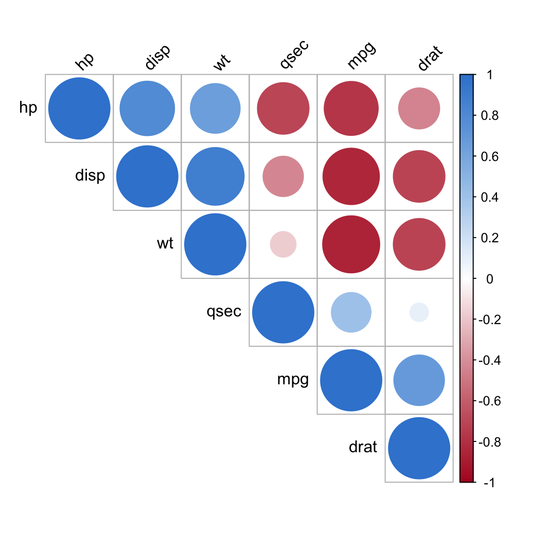
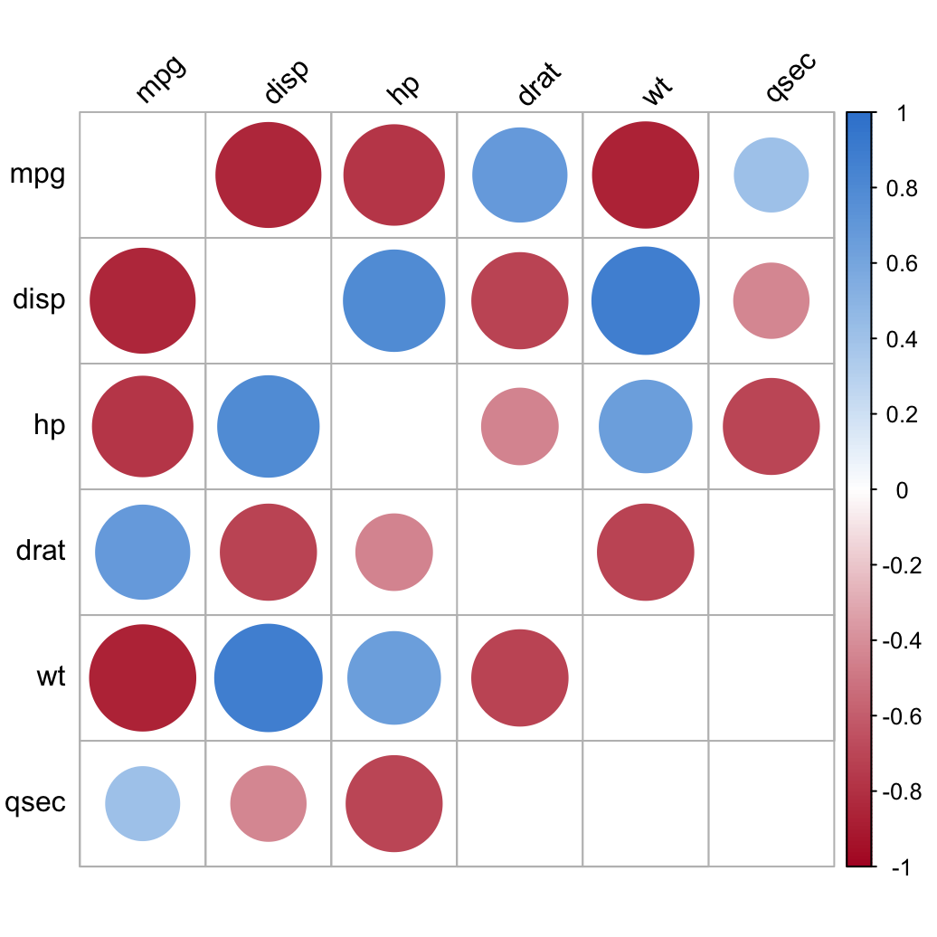
A correlogram turns the matrix into a picture: colour and size encode the coefficient. Reorder by clustering so related variables sit together, and show just the upper triangle:

library(corrplot)

mydata <- mtcars[, c("mpg", "disp", "hp", "drat", "wt", "qsec")]
res <- cor(mydata)

corrplot(
  res, type = "upper", order = "hclust",
  tl.col = "black", tl.srt = 45,
  col = colorRampPalette(c("#b2182b", "white", "#3a86d4"))(200)
)

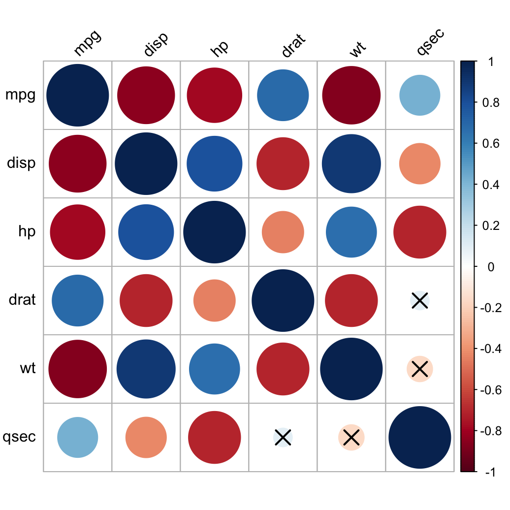
Positive correlations are blue, negative red; bigger, darker circles indicate stronger relationships. To blank out the insignificant cells, pass the p-value matrix:

library(corrplot)
library(Hmisc)

mydata <- mtcars[, c("mpg", "disp", "hp", "drat", "wt", "qsec")]
res <- cor(mydata)
p.mat <- rcorr(as.matrix(mydata))$P      # p-value matrix (Hmisc)
diag(p.mat) <- 0                          # mark the diagonal significant (avoids NA)

corrplot(
  res, p.mat = p.mat, sig.level = 0.05, insig = "blank",
  diag = FALSE, tl.col = "black", tl.srt = 45,
  col = colorRampPalette(c("#b2182b", "white", "#3a86d4"))(200)
)

Scatterplot matrix

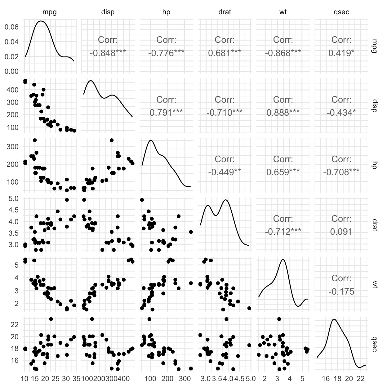
The most information-dense view pairs every variable with every other one. GGally::ggpairs() draws the distribution of each variable on the diagonal, the bivariate scatter plots below it, and the correlation coefficient with significance stars above it — the whole matrix as one picture:

library(GGally)

mydata <- mtcars[, c("mpg", "disp", "hp", "drat", "wt", "qsec")]
ggpairs(mydata) + theme_minimal()

Bigger coefficients (and more stars) above the diagonal mark the stronger, more significant relationships, and the scatter below lets you eyeball the linearity Pearson assumes before you trust the coefficient. psych::pairs.panels() and PerformanceAnalytics::chart.Correlation() draw the same diagonal-distribution / scatter / coefficient layout in base graphics.

Other quick views

rstatix::cor_plot() is a tidy wrapper around corrplot() that takes a cor_mat() result directly — no need to drop down to base cor():

library(rstatix)

mydata <- mtcars[, c("mpg", "disp", "hp", "drat", "wt", "qsec")]
mydata %>% cor_mat() %>% cor_plot()

Base R also ships heatmap() for a clustered colour grid:

mydata <- mtcars[, c("mpg", "disp", "hp", "drat", "wt", "qsec")]
res <- cor(mydata)
col <- colorRampPalette(c("#b2182b", "white", "#3a86d4"))(20)
heatmap(res, col = col, symm = TRUE)

And symnum() replaces coefficients with symbols for a compact text view:

mydata <- mtcars[, c("mpg", "disp", "hp", "drat", "wt", "qsec")]
res <- cor(mydata)
symnum(res, abbr.colnames = FALSE)

     mpg disp hp drat wt qsec
mpg  1                       
disp +   1                   
hp   ,   ,    1              
drat ,   ,    .  1           
wt   +   +    ,  ,    1      
qsec .   .    ,          1   
attr(,"legend")
[1] 0 ' ' 0.3 '.' 0.6 ',' 0.8 '+' 0.9 '*' 0.95 'B' 1

The legend shows the cutoffs: a blank for |r|<0.3, . to B for progressively stronger correlations. For deep correlogram customization (ordering, mixed methods, insignificance handling), see the dedicated correlogram lesson.

Try it live

Build and plot a correlation matrix on a different set of mtcars columns — add carb and gear, or swap the palette. The sandbox boots on first Run.

🟢 With an AI agent

Ask Prova “build a correlation matrix of my numeric columns and show me which ones are significant” — it answers with rstatix code you can run on your own data, then helps you read the correlogram. The runtime is the judge. Ask Prova →

Common issues

cor() errors on a data frame with text columns. A correlation matrix needs numeric input — select only numeric columns first (mydata[, sapply(mydata, is.numeric)]) or dplyr::select() them.

The matrix is full of NA. Missing values propagate. Add use = "complete.obs" to cor() (case-wise deletion) or clean the data before computing.

corrplot can’t blank insignificant cells. corrplot() needs a p-value matrix via p.mat =; cor() doesn’t produce one — get it from ggpubr::cor_pmat(), rstatix::cor_mat() |> cor_get_pval(), or Hmisc::rcorr()$P.

Frequently asked questions

NoteHow do I create a correlation matrix in R?

Use cor() from base R for the coefficients — cor(mydata) on a numeric data frame — or mydata %>% cor_mat() from rstatix for a tidy matrix that also carries the p-values. Round base-R output with round(cor(mydata), 2) for readability.

NoteHow do I get p-values for a correlation matrix?

Base cor() returns only coefficients. Use Hmisc::rcorr(as.matrix(mydata)) (its $P element is the p-value matrix), ggpubr::cor_pmat(mydata), or rstatix cor_mat() %>% cor_get_pval(). To combine coefficients and significance in one table, use rstatix::cor_mark_significant().

NoteWhat is a correlogram in R?

A correlogram is a graphical display of a correlation matrix where colour — and, with corrplot, circle size — encodes each pair’s correlation, so you can scan for the strongest and most significant relationships at a glance instead of reading a table of numbers. corrplot::corrplot() is the standard tool; rstatix::cor_plot() is a tidy wrapper that draws one straight from a cor_mat() result.

NoteHow do I visualize a correlation matrix in R?

The most popular way is a correlogram with corrplot::corrplot(cor(mydata), type = "upper") — colour and circle size encode the correlations. Other options are rstatix::cor_plot() (a tidy wrapper), base heatmap(), and symnum() for a compact symbol view.

NoteWhat is the difference between a correlation test and a correlation matrix?

A correlation test evaluates the relationship between two specific variables (coefficient + p-value + confidence interval). A correlation matrix computes the coefficient for every pair of numeric variables at once, giving a square table you scan or plot to compare many relationships.

NoteHow do I compute a Spearman correlation matrix in R?

Add the method argument: cor(mydata, method = "spearman") in base R, or mydata %>% cor_mat(method = "spearman") with rstatix (use "kendall" for Kendall’s tau). Spearman and Kendall work on ranks, so they capture monotonic relationships and are robust to non-normal or ordinal data — the same parametric-vs-rank choice as the two-variable correlation test.

NoteHow do I reorder or cluster a correlation matrix?

Pass order = "hclust" to corrplot() to reorder the variables by hierarchical clustering, so strongly related variables sit next to each other. For the table form, rstatix::cor_reorder() reorders a cor_mat() result the same way.

Test your understanding

ImportantPractice

1. Run it. In the live cell, compute a correlation matrix of mpg, wt, hp and qsec, then mark the significant correlations. Which pair is the strongest?
2. Conceptual. Your correlogram shows a strong blue circle between two variables, but blanking by sig.level = 0.05 leaves that cell empty. How can a large coefficient be non-significant?

NoteHint

Fill the four blanks with mpg, wt, hp, qsec. The strongest correlation has the coefficient closest to ±1 and the most stars. For question 2, think about sample size — significance depends on both the coefficient and how many observations you have.

NoteSolution

library(rstatix)
mtcars %>%
  select(mpg, wt, hp, qsec) %>%
  cor_mat() %>%
  cor_mark_significant()
#> mpg–wt is the strongest (r ≈ -0.87, ***).

For question 2: significance depends on the sample size, not just the coefficient. With few observations, even a large r can have a p-value above 0.05 (the confidence interval is wide), so corrplot blanks it. Collect more data, or report the coefficient with its interval rather than relying on the star alone.

Conclusion

You can now compute a correlation matrix in R the tidy rstatix way (cor_mat(), with p-values, reshaping and significance marks) and the classic base way (cor() + Hmisc::rcorr()), then turn it into a correlogram with corrplot() that highlights the strongest, significant relationships.

This closes the loop on the correlation test: test one pair, then scan them all. Next, revisit the assumption behind Pearson in the normality test lesson.

Related lessons

• Correlation test in R — the two-variable test (Pearson/Spearman/Kendall). · Normality test in R — the Shapiro-Wilk + Q-Q assumption check. · Scatter plots with correlation (ggpubr) — plot a single pair with stat_cor().
• Go further: The Correlation series — all correlation lessons in order. · Biostatistics — the full pillar.

Was this page helpful?

Prove you can do it. Master the whole Correlation in R series — track your path, build projects, and earn a certificate.

Start free →

Go Pro — unlimited Prova on your own data and a verifiable certificate that proves the skill.

from $15/mo billed yearly

Go Pro →

✓ You're Pro — keep going. The runtime is the judge.

Ready to level up?

Try this on your own data with Prova — the runtime is the judge.Open Prova →

Get new R & Python lessons by email

Practical, reproducible, no spam. Unsubscribe anytime.

Double opt-in. We never share your email.

Share this pageXLinkedInRedditHN

Note

Every result on this page was produced by the code shown, run at build time against a pinned R environment — edit any block and Run to reproduce it yourself.