Restricted Mean Survival Time (RMST) in R: An Interpretable Alternative to the Hazard Ratio

Q: What is restricted mean survival time (RMST)?

RMST is the area under the survival curve from time 0 to a horizon τ — equivalently, the expected survival time within the first τ units of follow-up. If a treated arm has RMST = 1450 days over 5 years, patients on that arm live, on average, 1450 of the first 1825 days. It is restricted because censoring makes the curve’s tail (and the true unrestricted mean) inestimable, so we stop at τ. The treatment effect is the difference or ratio of the two arms’ RMST.

Q: RMST vs hazard ratio — when should I use which?

Use the hazard ratio when proportional hazards holds and you want a conventional relative effect. Use RMST when you want an absolute, interpretable benefit (“months gained over τ”), or when the proportional-hazards assumption fails (curves cross, a delayed effect, a significant cox.zph()) — a single HR is then a misleading time-average, while RMST makes no PH assumption. In practice many trials now report both: the HR for the relative effect and the RMST difference for the absolute one.

Q: How do I choose tau for an RMST analysis?

Pick τ inside the support of both arms — at or below the smaller of the two arms’ maximum follow-up times — so you are not extrapolating a flat tail. Then prespecify it from the clinical question (e.g. 5-year survival → τ = 5 years), before looking at the results. τ defines the estimand, so it changes the answer: on the colon data, τ = 5 years gives a significant 111-day gain, but τ = 3 years gives only 31 days and p = 0.18. Choosing the τ that minimises p is fishing — fix it in advance.

Q: How do I compute RMST in R?

Use survRM2::rmst2(time, status, arm, tau = τ), where arm is a 0/1 vector. It returns the per-arm RMST and the between-group difference and ratio, each with a 95% CI and p-value. For just the per-arm numbers you can also call print(survfit(Surv(time, status) ~ group, data), rmean = τ) and read the rmean* column — but survfit alone gives no contrast, CI, or p-value, so use rmst2() to test the treatment effect.

Q: Does RMST assume proportional hazards?

No. RMST simply compares the area under each arm’s survival curve up to τ; it never assumes the hazard ratio is constant. That is exactly why it is recommended when proportional hazards fails — where a single hazard ratio is a misleading average, the RMST difference remains a valid, interpretable summary of the effect. Pair it with a weighted log-rank test for a more powerful p-value in the non-PH setting.

Measure a treatment effect in months gained, not an abstract hazard ratio — compute the area under the survival curve up to a horizon with survRM2::rmst2(), get the RMST difference and ratio with 95% CI and p, and use it when proportional hazards fail

Biostatistics

Compute the restricted mean survival time (RMST) in R — the area under the survival curve up to a horizon tau, the expected survival time within the first tau units. Estimate the per-arm RMST and the between-group difference and ratio with 95% confidence intervals and a p-value using survRM2::rmst2() (and the rmean from survfit), choose tau within the support of both arms, draw the signature shaded-area survival plot, and learn when to report RMST instead of a hazard ratio — for an absolute clinical benefit, or when the proportional-hazards assumption fails.

Published

June 26, 2026

Modified

July 7, 2026

Key takeaways

Restricted mean survival time (RMST) is the area under the survival curve from 0 to a horizon τ — equivalently, the expected survival time within the first τ units. It is reported in real time units (“patients live, on average, 1450 days over 5 years”), so it is directly interpretable.
The treatment effect is the RMST difference (arm 1 minus arm 0, “X days/months gained on average over τ”) or the RMST ratio — both with a 95% CI and a p-value. Unlike a single hazard ratio, RMST does not assume proportional hazards, so it is valid when curves cross or the effect is delayed.
Compute it with survRM2::rmst2(time, status, arm, tau = …): it returns the per-arm RMST and the between-group difference and ratio. The per-arm RMST also comes free from print(survfit(...), rmean = τ).
Choose τ before you look at the results, inside the support of both arms (roughly, the smaller arm’s largest follow-up time). On the colon-cancer data, τ = 5 years gives a 111-day (≈ 3.7-month) gain, p = 0.018; the same comparison at τ = 3 years is only 31 days and not significant — the horizon matters, so prespecify it.
Reach for RMST when you want an absolute, clinically interpretable benefit instead of a hazard ratio, or when the proportional-hazards assumption fails and a single HR is misleading.

Introduction

A hazard ratio of 0.69 is a fine number for a statistician and a terrible one for a patient. “Your instantaneous risk of death is reduced by 31%” answers a question almost no one asked, and it only means anything if that 31% holds at every moment of follow-up — the proportional-hazards assumption. When immunotherapy curves separate only after a year, or two curves cross, that single ratio is a misleading time-average and the question “so how much longer do people actually live?” goes unanswered.

Restricted mean survival time (RMST) answers exactly that question. It is the area under the survival curve up to a horizon τ — the average survival time a patient can expect within the first τ units of follow-up. The treatment effect becomes a difference of two areas: “patients on the new drug live, on average, 3.7 months longer over 5 years.” That sentence needs no statistical translation, and — crucially — it stays valid even when proportional hazards do not, because it never assumes a constant ratio.

This lesson computes RMST in R on a real two-arm trial, using survival and survRM2 (Uno et al.). You will:

understand RMST as the area under S(t) up to τ, and why that makes it interpretable and PH-free;
compute the per-arm RMST and the RMST difference and ratio with 95% CI and a p-value via rmst2();
choose τ correctly (inside the support of both arms) and see why it changes the answer;
draw the signature shaded-area figure;
and know when to report RMST instead of a hazard ratio.

What RMST measures

For a survival function $S(t)$ and a fixed horizon $\tau$, the restricted mean survival time is

\[ \text{RMST}(\tau) = \int_{0}^{\tau} S(t)\, dt \]

— the area under the survival curve up to τ. Because $S(t)$ is the Kaplan-Meier estimate, this is just the area under the KM step function, capped at τ. It is restricted because we stop at τ (survival data are censored, so the curve’s tail — and the true mean — are not estimable). The treatment effect is the difference $\text{RMST}_1(\tau) - \text{RMST}_0(\tau)$ or the ratio, each a hypothesis you can test.

When to reach for RMST

RMST is not a replacement for the hazard ratio everywhere — it is the right tool for two specific jobs:

You want an absolute, clinically interpretable benefit. A hazard ratio is relative and abstract; “4 months gained over 2 years” is absolute and concrete. Regulators and clinicians increasingly ask for RMST alongside (or instead of) the HR for this reason.
The proportional-hazards assumption fails. When the PH check (cox.zph()) is significant, the curves cross, or the effect is delayed, a single hazard ratio is a misleading average. RMST makes no PH assumption — it just compares two areas — so it stays valid. It is a natural companion to a weighted log-rank test: the weighted test gives a more powerful p-value for “do the curves differ?”, and RMST gives the effect size in time units.

RMST is a summary, not a magic fix

RMST collapses the whole curve up to τ into one number. That is its strength (interpretability) and its limit: it cannot tell you when the benefit accrues, and two very different curves can share an RMST. Pair it with the Kaplan-Meier plot so the reader sees the shape, and prespecify τ from the clinical question — not from the data.

The data: a two-arm colon-cancer trial

We use colon, the adjuvant chemotherapy trial that ships with the survival package. Each patient appears twice (recurrence and death); we keep the death records (etype == 2) and compare two arms: observation (Obs) versus levamisole + 5-FU (Lev+5FU), the effective regimen. With survival attached the data is available directly — no data() call needed. rmst2() needs the arm coded 0/1, so we build that in the same block:

library(survival)

# Death records (etype == 2), two arms: observation vs Lev+5FU
dat <- subset(colon, etype == 2 & rx %in% c("Obs", "Lev+5FU"))
dat$rx <- droplevels(dat$rx)

# survRM2 needs a 0/1 arm: 1 = treated (Lev+5FU), 0 = observation
arm <- ifelse(dat$rx == "Lev+5FU", 1, 0)

c(n = nrow(dat), events = sum(dat$status), treated = sum(arm), control = sum(arm == 0))

      n  events treated control 
    619     291     304     315

time — follow-up time in days; status — 1 = death, 0 = censored.
arm — 1 = Lev+5FU (304 patients), 0 = observation (315 patients); 291 deaths in total.

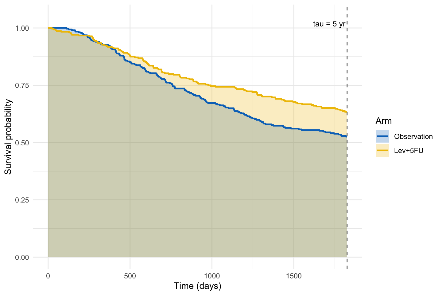
Look at the curves first. The treated curve should sit above observation — and the gap between the two areas up to a horizon is exactly the RMST gain we are about to quantify.

library(survival)
library(ggplot2)

dat <- subset(colon, etype == 2 & rx %in% c("Obs", "Lev+5FU"))
dat$rx <- droplevels(dat$rx)

tau <- 1825                                   # 5-year horizon (days)
fit <- survfit(Surv(time, status) ~ rx, data = dat)

# Build a step polygon per arm, clipped at tau, so geom_area shades the AREA = RMST
arms <- rep(names(fit$strata), fit$strata)
sd   <- data.frame(time = fit$time, surv = fit$surv, arm = sub("rx=", "", arms))

step_poly <- function(s) {
  s <- s[order(s$time), ]
  s <- s[s$time <= tau, ]
  t <- c(0, rep(s$time, each = 2), tau)
  v <- c(1, 1, rep(s$surv, each = 2))
  v <- v[seq_len(length(t))]
  data.frame(time = t, surv = v, arm = s$arm[1])
}
poly <- do.call(rbind, lapply(split(sd, sd$arm), step_poly))
poly$arm <- factor(poly$arm, levels = c("Obs", "Lev+5FU"),
                   labels = c("Observation", "Lev+5FU"))

ggplot(poly, aes(time, surv)) +
  geom_area(aes(fill = arm), alpha = 0.25, position = "identity") +
  geom_step(aes(colour = arm), linewidth = 0.9, direction = "hv") +
  geom_vline(xintercept = tau, linetype = "dashed", colour = "grey40") +
  annotate("text", x = tau, y = 1.02, label = "tau = 5 yr", hjust = 1.05, size = 3.3) +
  scale_fill_manual(values = c("#0073C2", "#EFC000")) +      # jco palette
  scale_colour_manual(values = c("#0073C2", "#EFC000")) +
  scale_y_continuous(limits = c(0, 1.05)) +
  labs(x = "Time (days)", y = "Survival probability",
       fill = "Arm", colour = "Arm") +
  theme_minimal()

Two Kaplan-Meier survival curves for a colon-cancer trial, observation in blue and Lev+5FU in gold, with the area under each curve shaded up to a dashed vertical line at five years. The gold treated curve sits above the blue observation curve from about 300 days onward, and the extra gold sliver between the two curves is the gain in restricted mean survival time. The shaded area under each curve up to tau is that arm's RMST.

The shaded area under each curve up to τ is that arm’s RMST. The gold (Lev+5FU) area is visibly larger than the blue (observation) area; the extra gold sliver between the curves is the RMST difference — the average survival time the treatment buys over five years. Now we put a number on it.

Compute RMST with `survRM2::rmst2()`

rmst2() takes three vectors — the survival time, the event status, and the arm (0/1) — plus the horizon tau. It returns the RMST for each arm and the between-group contrast (difference and ratio). Run it at the five-year horizon:

library(survival)
library(survRM2)

dat <- subset(colon, etype == 2 & rx %in% c("Obs", "Lev+5FU"))
dat$rx <- droplevels(dat$rx)
arm <- ifelse(dat$rx == "Lev+5FU", 1, 0)

res <- rmst2(dat$time, dat$status, arm, tau = 1825)
res


The truncation time: tau = 1825  was specified. 

Restricted Mean Survival Time (RMST) by arm 
                 Est.     se lower .95 upper .95
RMST (arm=1) 1449.880 32.998  1385.205  1514.556
RMST (arm=0) 1338.549 33.441  1273.005  1404.093


Restricted Mean Time Lost (RMTL) by arm 
                Est.     se lower .95 upper .95
RMTL (arm=1) 375.120 32.998   310.444   439.795
RMTL (arm=0) 486.451 33.441   420.907   551.995


Between-group contrast 
                        Est. lower .95 upper .95     p
RMST (arm=1)-(arm=0) 111.332    19.250   203.413 0.018
RMST (arm=1)/(arm=0)   1.083     1.014     1.157 0.018
RMTL (arm=1)/(arm=0)   0.771     0.620     0.960 0.020

Read the output top to bottom:

RMST by arm — over the first 5 years a treated patient (arm = 1) survives 1450 days on average (95% CI 1385–1515); an observation patient (arm = 0) survives 1339 days (95% CI 1273–1404). These are real, interpretable expected survival times within the horizon.
RMTL by arm — the restricted mean time lost, $\tau - \text{RMST}$: the average time not survived within τ (375 vs 486 days). It is the mirror image of RMST and sometimes reported instead.
Between-group contrast — three rows:
- RMST difference (arm 1 − arm 0) = 111.3 days (95% CI 19.3–203.4), p = 0.018. Treated patients live, on average, about 111 days — roughly 3.7 months — longer over 5 years, and the CI excludes 0, so the gain is significant.
- RMST ratio = 1.083 (95% CI 1.014–1.157, p = 0.018) — an 8.3% larger restricted mean survival.
- RMTL ratio = 0.771 — treated patients lose 23% less of the 5 years.

That is the whole result in plain language: 3.7 more months of life, on average, over the first five years — a number a patient understands, with no hazard ratio in sight.

The same per-arm RMST from `survfit`

You do not strictly need a package for the per-arm numbers — base survfit reports the restricted mean when you ask print() for rmean:

library(survival)

dat <- subset(colon, etype == 2 & rx %in% c("Obs", "Lev+5FU"))
dat$rx <- droplevels(dat$rx)

fit <- survfit(Surv(time, status) ~ rx, data = dat)
print(fit, rmean = 1825)

Call: survfit(formula = Surv(time, status) ~ rx, data = dat)

             n events rmean* se(rmean) median 0.95LCL 0.95UCL
rx=Obs     315    168   1339      33.4   2083    1656    2789
rx=Lev+5FU 304    123   1450      33.0     NA    2725      NA
    * restricted mean with upper limit =  1825

The rmean* column reads 1339 for observation and 1450 for Lev+5FU — identical to rmst2()’s per-arm RMST (the asterisk footnote names the upper limit, τ = 1825). What rmst2() adds is the inferential contrast — the difference, the ratio, the CIs and the p-value — which survfit alone does not give. Use survfit for a quick per-arm read, rmst2() to test the treatment effect.

Choosing τ — the one decision that matters

τ is not a nuisance parameter; it defines the estimand, so it changes the answer. Two rules:

1. τ must lie inside the support of both arms. RMST integrates the KM curve up to τ, and the curve is only estimable up to the last follow-up time in each arm. Push τ past the smaller arm’s largest time and you are extrapolating a flat tail — the estimate becomes unstable and the variance unreliable. A safe default is at or below the smaller of the two arms’ maximum event/censoring times (here both arms follow patients past 5 years, so τ = 1825 days is comfortably inside).

2. Prespecify τ from the clinical question — never tune it. The horizon you pick is the window over which you are measuring benefit. Watch what happens if we ask for a 3-year horizon instead:

library(survival)
library(survRM2)

dat <- subset(colon, etype == 2 & rx %in% c("Obs", "Lev+5FU"))
dat$rx <- droplevels(dat$rx)
arm <- ifelse(dat$rx == "Lev+5FU", 1, 0)

res3 <- rmst2(dat$time, dat$status, arm, tau = 1095)   # 3-year horizon
res3$unadjusted.result

                           Est.   lower .95 upper .95         p
RMST (arm=1)-(arm=0) 30.7322857 -14.1253539 75.589925 0.1793415
RMST (arm=1)/(arm=0)  1.0334761   0.9849630  1.084379 0.1794922
RMTL (arm=1)/(arm=0)  0.8263345   0.6236949  1.094812 0.1838769

At τ = 3 years the RMST difference is only 30.7 days with p = 0.18 — not significant. The curves barely separate in the first three years and pull apart later, so a short horizon misses most of the benefit. Same data, same arms, different conclusion — purely because of τ. That is exactly why τ must be fixed in advance from the clinical question (here, 5-year survival), not chosen to make the p-value small. Reporting the τ that minimises p is the RMST version of fishing.

Report

Pull the three numbers a paper needs straight from the result object:

library(survival)
library(survRM2)

dat <- subset(colon, etype == 2 & rx %in% c("Obs", "Lev+5FU"))
dat$rx <- droplevels(dat$rx)
arm <- ifelse(dat$rx == "Lev+5FU", 1, 0)

res <- rmst2(dat$time, dat$status, arm, tau = 1825)
rmst_treated <- round(res$RMST.arm1$result["RMST", "Est."])
rmst_control <- round(res$RMST.arm0$result["RMST", "Est."])
diff_row     <- res$unadjusted.result[1, ]             # difference: Est. + 95% CI + p

c(rmst_treated = rmst_treated, rmst_control = rmst_control)

rmst_treated rmst_control 
        1450         1339

round(diff_row[1:3], 1)                                # difference in days + 95% CI

     Est. lower .95 upper .95 
    111.3      19.3     203.4

signif(diff_row[4], 3)                                 # p-value (kept at full precision)

     p 
0.0178

Treatment effect was summarised with the restricted mean survival time over a prespecified 5-year horizon (τ = 1825 days) on the colon-cancer trial (n = 619, 291 deaths). Patients receiving Lev+5FU had a restricted mean survival of 1450 days versus 1339 days under observation, a difference of 111 days (≈ 3.7 months; 95% CI 19–203 days, p = 0.018) in favour of treatment (RMST ratio 1.08, 95% CI 1.01–1.16). Because RMST makes no proportional-hazards assumption, this absolute survival gain is reported alongside the hazard ratio.

The math behind RMST (optional)

For a survival function $S(t)$ and horizon $\tau$, the restricted mean survival time is the area under the curve:

\[ \mu(\tau) = \int_{0}^{\tau} S(t)\, dt \]

This is the restricted expectation $E[\min(T, \tau)]$ — the expected value of survival time capped at τ. (The unrestricted mean $E[T] = \int_0^\infty S(t)\,dt$ is the area under the whole curve, but with censoring the tail of $S$ is not estimable, which is why we restrict to τ.) Plugging in the Kaplan-Meier estimate $\hat S(t)$, the integral becomes a sum of rectangles — the KM step function is piecewise constant, so

\[ \hat\mu(\tau) = \sum_{k} \hat S(t_{k-1}) \,(t_k - t_{k-1}) \]

over the event times up to τ. The variance comes from Greenwood-type plug-in (Uno et al. 2014), giving the 95% CIs rmst2() reports. The difference $\hat\mu_1(\tau) - \hat\mu_0(\tau)$ and its CI are then a straightforward two-sample comparison — and at no point did we assume the hazard ratio is constant, which is the whole reason RMST survives non-proportional hazards.

RMST vs the hazard ratio — which to report

Pick the summary by the question and the assumption

Proportional hazards holds, and you want a relative effect → the hazard ratio (Cox model) is the efficient, conventional summary.
You want an absolute, interpretable benefit (“how many months?”) → RMST difference, reported alongside the HR.
Proportional hazards fails (the PH check is significant, curves cross, or the effect is delayed) → a single HR is a misleading average; report RMST (effect size) and, for the test, a weighted log-rank p-value.
You need to know when the benefit accrues → neither single number suffices; show the Kaplan-Meier curves and consider a time-varying Cox model.

Try it live

Compute RMST yourself — change τ, swap the arms, or try the observation-vs-levamisole comparison. The sandbox boots on first Run.

🟢 With an AI agent

Ask Prova “compute the restricted mean survival time for my two-arm trial in R with survRM2, give me the RMST difference in months with its 95% CI and p-value, and tell me whether to report it instead of the hazard ratio” — it answers with survival + survRM2 code you can run on your own data. The runtime is the judge. Ask Prova →

Common issues

You set τ beyond the smaller arm’s last follow-up time. RMST integrates the KM curve up to τ, but the curve is only estimable up to each arm’s largest observed time. Push τ past the shorter arm’s support and rmst2() extrapolates a flat tail — the estimate drifts and its variance is unreliable (newer versions warn or error). Set τ at or below the smaller of the two arms’ maximum times; check with tapply(dat$time, arm, max).

You compared RMST values computed at different τ. RMST is only defined for a given τ — a difference at τ = 3 years and one at τ = 5 years are answering different questions and are not comparable. Fix one prespecified τ for the whole analysis and report it explicitly.

Your arm isn’t coded 0/1. rmst2() requires the arm argument to be a numeric 0/1 vector (two groups only). A factor (Obs/Lev+5FU), a 1/2 coding, or three or more levels will error or mislabel the contrast. Build it with ifelse(group == "treated", 1, 0) and confirm with table(arm). For more than two arms, run RMST pairwise (and adjust for multiple comparisons).

Frequently asked questions

What is restricted mean survival time (RMST)?

RMST is the area under the survival curve from time 0 to a horizon τ — equivalently, the expected survival time within the first τ units of follow-up. If a treated arm has RMST = 1450 days over 5 years, patients on that arm live, on average, 1450 of the first 1825 days. It is restricted because censoring makes the curve’s tail (and the true unrestricted mean) inestimable, so we stop at τ. The treatment effect is the difference or ratio of the two arms’ RMST.

RMST vs hazard ratio — when should I use which?

Use the hazard ratio when proportional hazards holds and you want a conventional relative effect. Use RMST when you want an absolute, interpretable benefit (“months gained over τ”), or when the proportional-hazards assumption fails (curves cross, a delayed effect, a significant cox.zph()) — a single HR is then a misleading time-average, while RMST makes no PH assumption. In practice many trials now report both: the HR for the relative effect and the RMST difference for the absolute one.

How do I choose tau for an RMST analysis?

Pick τ inside the support of both arms — at or below the smaller of the two arms’ maximum follow-up times — so you are not extrapolating a flat tail. Then prespecify it from the clinical question (e.g. 5-year survival → τ = 5 years), before looking at the results. τ defines the estimand, so it changes the answer: on the colon data, τ = 5 years gives a significant 111-day gain, but τ = 3 years gives only 31 days and p = 0.18. Choosing the τ that minimises p is fishing — fix it in advance.

How do I compute RMST in R?

Use survRM2::rmst2(time, status, arm, tau = τ), where arm is a 0/1 vector. It returns the per-arm RMST and the between-group difference and ratio, each with a 95% CI and p-value. For just the per-arm numbers you can also call print(survfit(Surv(time, status) ~ group, data), rmean = τ) and read the rmean* column — but survfit alone gives no contrast, CI, or p-value, so use rmst2() to test the treatment effect.

Does RMST assume proportional hazards?

No. RMST simply compares the area under each arm’s survival curve up to τ; it never assumes the hazard ratio is constant. That is exactly why it is recommended when proportional hazards fails — where a single hazard ratio is a misleading average, the RMST difference remains a valid, interpretable summary of the effect. Pair it with a weighted log-rank test for a more powerful p-value in the non-PH setting.

Test your understanding

Practice

Run it. In the live cell below, compute RMST at a 3-year horizon (τ = 1095) for the same two arms. Fill the blank. Is the RMST difference significant at 3 years? Compare it to the 5-year result in the lesson and explain the change.
Interpret. A trial reports an RMST difference of +2.8 months (95% CI 0.4 to 5.2, p = 0.02) over a 2-year horizon, with a non-significant hazard ratio because the curves cross. Write one plain-language sentence a patient would understand, and say why RMST is the better summary here.

Hint

Fill the blank with 1095 (3 years in days). Read the first row, RMST (arm=1)-(arm=0): the Est. column is the difference in days and the last column is the p-value. Compare it to the 5-year difference (111 days, p = 0.018) — the curves separate late, so a shorter horizon captures less of the benefit.

Solution

res <- rmst2(dat$time, dat$status, arm, tau = 1095)
res$unadjusted.result
#> RMST (arm=1)-(arm=0)  Est. = 30.7 days, 95% CI roughly -14 to 75, p = 0.18 — NOT significant.
#> At a 3-year horizon the treated and observation curves have barely separated, so the area
#> between them is small. The benefit accrues LATER, which is why the 5-year horizon (111 days,
#> p = 0.018) is significant and the 3-year one is not. The conclusion depends on tau — so tau
#> must be prespecified from the clinical question, not chosen to make p small.

For question 2: “On average, patients on the new treatment lived about 2.8 months longer over the two years of the study (95% CI 0.4 to 5.2 months).” RMST is the better summary because the curves cross, so proportional hazards fails and the single hazard ratio is a misleading time-average — RMST makes no PH assumption and reports the benefit as an interpretable, absolute amount of time.

Quick check

A reviewer asks you to report RMST at “whichever τ gives the clearest result.” You try τ = 2, 3, 4, and 5 years and report the τ with the smallest p-value. What is wrong with this?

Show answer

It is fishing. τ defines the estimand, so trying several horizons and reporting the one that minimises p inflates the type-I error rate exactly like trying many tests — you will “find” significance that isn’t robust. τ must be prespecified from the clinical question (e.g. the trial’s primary follow-up window) before seeing the results; the others are at most prespecified sensitivity analyses, not a menu to pick the winner from.

Conclusion

Restricted mean survival time turns a survival comparison into a number anyone can act on. It is the area under the survival curve up to a horizon τ — the average survival time within the first τ units — and the treatment effect is the difference of two areas, reported in real time units with a 95% CI and a p-value. Compute it with survRM2::rmst2(time, status, arm, tau = …) (the per-arm RMST also falls out of print(survfit(...), rmean = τ)). On the colon-cancer trial, Lev+5FU bought 111 days — about 3.7 months — of extra survival over 5 years (p = 0.018); the same comparison at 3 years was not significant, a reminder that τ defines the estimand and must be prespecified. Reach for RMST when you want an absolute, clinically interpretable benefit, or when the proportional-hazards assumption fails and a single hazard ratio would mislead — there, RMST gives you the effect size that the hazard ratio cannot.

Reuse

CC BY-NC-SA 4.0

Citation

BibTeX citation:

@online{2026,
  author = {},
  title = {Restricted {Mean} {Survival} {Time} {(RMST)} in {R:} {An}
    {Interpretable} {Alternative} to the {Hazard} {Ratio}},
  date = {2026-06-26},
  url = {https://www.datanovia.com/learn/biostatistics/survival-analysis/rmst},
  langid = {en}
}

For attribution, please cite this work as:

“Restricted Mean Survival Time (RMST) in R: An Interpretable Alternative to the Hazard Ratio.” 2026. June 26. https://www.datanovia.com/learn/biostatistics/survival-analysis/rmst.