Logistic Regression in R: Model a Binary Outcome

Q: How do I run a logistic regression in R?

Use glm(y ~ x, family = binomial) with a binary outcome y. Summarize with summary(model), get interpretable effects with exp(coef(model)) (odds ratios), and predict probabilities with predict(model, newdata, type = "response").

Q: How do I interpret logistic regression coefficients / odds ratios?

A coefficient is the change in log-odds per unit of the predictor — not directly meaningful. Take exp(coefficient) to get the odds ratio: OR > 1 means the predictor raises the odds of the outcome, OR < 1 lowers them, OR = 1 means no effect. An OR of 1.04 means a 4% increase in odds per unit.

Q: What is the difference between logistic and linear regression?

Linear regression predicts a numeric outcome with an unbounded straight line; logistic regression predicts the probability of a binary outcome through an S-shaped curve bounded in [0, 1]. Logistic models the log-odds (logit) and is fit by maximum likelihood with a z-test, not least squares with a t-test.

Q: How do I get predicted probabilities from a logistic model?

Use predict(model, newdata, type = "response") — the type = "response" is essential, or you get log-odds instead of probabilities. The result is the probability of the outcome level coded 1 (check with contrasts()).

Predict a yes/no outcome with glm(family = binomial), interpret the coefficients as odds ratios, read the log-odds, and get the probability curve — the practical, interpretation-first way

Biostatistics

Learn logistic regression in R — model a binary (yes/no) outcome with glm(family = binomial). Fit simple and multiple models, interpret the coefficients as odds ratios with confidence intervals, understand log-odds/logit, predict class probabilities, and read the S-shaped probability curve. Interpretation-first.

Published

June 23, 2026

Modified

July 7, 2026

Key takeaways

Logistic regression models a binary outcome (yes/no, 0/1, diseased/healthy) — it predicts the probability of the “1” class, not the class directly.
Fit it with glm(y ~ x, family = binomial) — a generalized linear model on the log-odds (logit) of the outcome.
A coefficient is the change in log-odds per unit of the predictor; exp(coef) is the odds ratio — the interpretable effect (OR > 1 raises the odds, OR < 1 lowers them).
Predict probabilities with predict(model, newdata, type = "response"); the S-shaped curve maps the linear predictor to a 0–1 probability.
This is the inference view — interpret which predictors matter and by how much. (Classification accuracy, cross-validation and variable selection belong to the Machine Learning pillar.)

Introduction

Linear regression models a numeric outcome — but many outcomes are binary: a patient is diabetic or not, a customer churns or not, a loan defaults or not. Logistic regression handles exactly this: it’s a generalized linear model (GLM) that predicts the probability of the “yes” class and lets you interpret each predictor as an odds ratio.

The scenario: from clinical measurements, model the probability of testing positive for diabetes — and read off which factors raise the odds, and by how much.

The data: clinical measurements

We use the PimaIndiansDiabetes2 dataset from the mlbench package — clinical variables (glucose, BMI, age, …) and a binary diabetes outcome (pos/neg). We drop incomplete rows:

data("PimaIndiansDiabetes2", package = "mlbench")
diabetes_data <- na.omit(PimaIndiansDiabetes2)

head(diabetes_data, 4)

  pregnant glucose pressure triceps insulin mass pedigree age diabetes
4        1      89       66      23      94 28.1    0.167  21      neg
5        0     137       40      35     168 43.1    2.288  33      pos
7        3      78       50      32      88 31.0    0.248  26      pos
9        2     197       70      45     543 30.5    0.158  53      pos

Simple logistic regression

Model the probability of diabetes from plasma glucose alone. glm() with family = binomial fits the logistic model:

data("PimaIndiansDiabetes2", package = "mlbench")
diabetes_data <- na.omit(PimaIndiansDiabetes2)

model <- glm(diabetes ~ glucose, data = diabetes_data, family = binomial)
summary(model)$coef

               Estimate  Std. Error   z value     Pr(>|z|)
(Intercept) -6.09552139 0.629787038 -9.678703 3.713993e-22
glucose      0.04242099 0.004760623  8.910805 5.066328e-19

The intercept is −6.10 and the glucose coefficient is 0.042 — positive, so higher glucose means higher diabetes probability. But the coefficient is on the log-odds scale, which isn’t directly interpretable. That’s what the odds ratio fixes.

Interpret with odds ratios

exp(coefficient) is the odds ratio — the multiplicative change in the odds of the outcome per one-unit increase in the predictor. This is the number you report:

data("PimaIndiansDiabetes2", package = "mlbench")
diabetes_data <- na.omit(PimaIndiansDiabetes2)
model <- glm(diabetes ~ glucose, data = diabetes_data, family = binomial)

exp(cbind(OR = coef(model), confint(model)))   # odds ratio + 95% CI

                     OR        2.5 %      97.5 %
(Intercept) 0.002252935 0.0006194309 0.007358113
glucose     1.043333616 1.0340267589 1.053554337

The glucose odds ratio is 1.04 (95% CI excludes 1) — each 1-unit increase in glucose multiplies the odds of diabetes by 1.04 (a 4% increase in odds per unit). Over a 50-unit glucose rise, that compounds to $1.04^{50} \approx 7\text{–}8$× the odds.

The probability curve

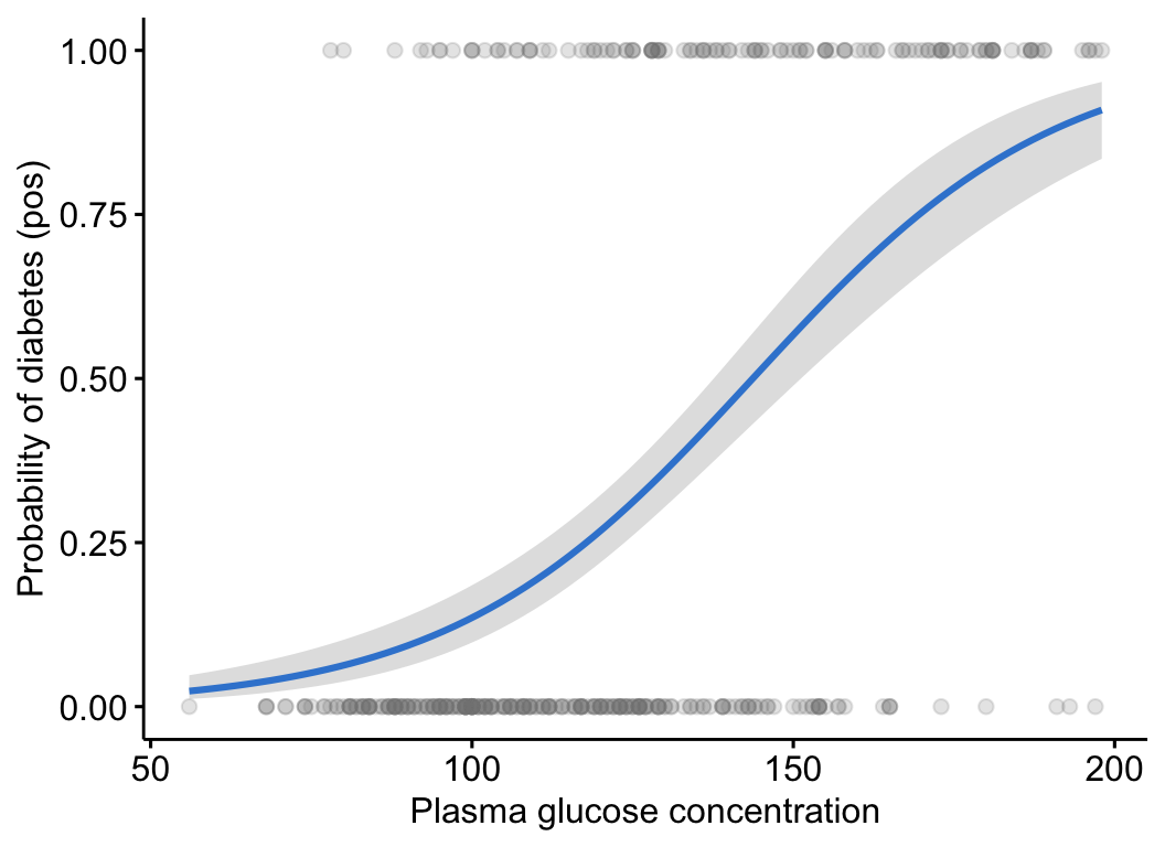
Logistic regression maps the linear predictor through an S-shaped curve into a 0–1 probability — the signature logistic shape:

library(ggpubr)

data("PimaIndiansDiabetes2", package = "mlbench")
diabetes_data <- na.omit(PimaIndiansDiabetes2)
diabetes_data$prob <- ifelse(diabetes_data$diabetes == "pos", 1, 0)

ggscatter(diabetes_data, x = "glucose", y = "prob", color = "grey50",
          alpha = 0.2, xlab = "Plasma glucose concentration",
          ylab = "Probability of diabetes (pos)") +
  geom_smooth(method = "glm", method.args = list(family = "binomial"),
              color = "#3a86d4", fill = "grey70")

An S-shaped logistic regression curve showing the probability of being diabetes-positive rising with plasma glucose concentration, plotted over the observed outcomes coded as 0 and 1.

The curve is near 0 at low glucose, rises steeply through the middle, and saturates near 1 — a probability always stays in [0, 1], unlike a straight line.

Multiple logistic regression

Add all the clinical predictors with ~ ., then read the odds ratios. broom::tidy() with exponentiate = TRUE gives the OR table with confidence intervals and p-values in one step:

library(broom)

data("PimaIndiansDiabetes2", package = "mlbench")
diabetes_data <- na.omit(PimaIndiansDiabetes2)

model <- glm(diabetes ~ ., data = diabetes_data, family = binomial)
tidy(model, exponentiate = TRUE, conf.int = TRUE)

# A tibble: 9 × 7
  term         estimate std.error statistic  p.value   conf.low conf.high
  <chr>           <dbl>     <dbl>     <dbl>    <dbl>      <dbl>     <dbl>
1 (Intercept) 0.0000436   1.22       -8.25  1.64e-16 0.00000355  0.000426
2 pregnant    1.09        0.0554      1.48  1.38e- 1 0.974       1.21    
3 glucose     1.04        0.00577     6.64  3.24e-11 1.03        1.05    
4 pressure    0.999       0.0118     -0.120 9.04e- 1 0.976       1.02    
5 triceps     1.01        0.0171      0.657 5.11e- 1 0.978       1.05    
6 insulin     0.999       0.00131    -0.632 5.28e- 1 0.997       1.00    
7 mass        1.07        0.0273      2.58  9.89e- 3 1.02        1.13    
8 pedigree    3.13        0.427       2.67  7.60e- 3 1.38        7.37    
9 age         1.03        0.0184      1.85  6.47e- 2 0.999       1.07

Read it as odds ratios, holding the other predictors constant:

glucose (OR ≈ 1.04, p < 0.001), mass/BMI (OR ≈ 1.07, p = 0.01) and pedigree (OR ≈ 3.13, p = 0.008) are significant — each raises the odds of diabetes. A family-history pedigree OR of 3.1 means a one-unit increase triples the odds.
pregnant, pressure, triceps, insulin and age are not significant here (their CIs include OR = 1) — no clear independent effect once the others are accounted for.

Note

Odds ratio, not probability. A coefficient’s exp() is an odds ratio (multiplicative effect on the odds), not a change in probability. OR > 1 raises the odds, OR < 1 lowers them, OR = 1 means no effect — and a CI that includes 1 means non-significant.

Predict probabilities

Use predict(..., type = "response") to get probabilities for new individuals (without type, predict returns log-odds):

data("PimaIndiansDiabetes2", package = "mlbench")
diabetes_data <- na.omit(PimaIndiansDiabetes2)
model <- glm(diabetes ~ glucose, data = diabetes_data, family = binomial)

newdata <- data.frame(glucose = c(90, 150, 200))
predict(model, newdata, type = "response")

         1          2          3 
0.09299244 0.56651015 0.91595970

A glucose of 90 gives a low diabetes probability; 200 gives a high one. Which class does the probability refer to? Check the dummy coding — R models the probability of the level coded 1:

data("PimaIndiansDiabetes2", package = "mlbench")
diabetes_data <- na.omit(PimaIndiansDiabetes2)

contrasts(diabetes_data$diabetes)     # 'pos' is coded 1 -> the modelled probability

    pos
neg   0
pos   1

Report

A logistic regression modelled the probability of a positive diabetes test from clinical predictors. Glucose (OR = 1.04 per unit, 95% CI 1.03–1.05, p < 0.001), BMI (OR = 1.07, p = 0.01) and diabetes pedigree (OR = 3.13, 95% CI 1.38–7.37, p = 0.008) were significant positive predictors of diabetes, adjusting for the other variables.

The math (optional): the logit link

Logistic regression models the log-odds (logit) of the outcome as linear in the predictors: $\log\!\dfrac{p}{1-p} = \beta_0 + \beta_1 x_1 + \dots + \beta_k x_k$, where $p = P(y = 1 \mid x)$. Solving for $p$ gives the S-curve $p = \dfrac{1}{1 + e^{-(\beta_0 + \beta_1 x_1 + \dots)}}$, which always lies in $(0, 1)$. Because the model is linear in log-odds, $e^{\beta_j}$ is the odds ratio — the factor by which the odds multiply per unit of $x_j$. The coefficients are estimated by maximum likelihood, and significance uses a z-test (Pr(>|z|)) rather than the t-test of linear regression.

Try it live

Fit a different predictor — does BMI (mass) predict diabetes? Read its odds ratio. The sandbox boots on first Run.

🟢 With an AI agent

Ask Prova “fit a logistic regression on my binary outcome, interpret the odds ratios, and tell me which predictors matter” — it answers with code you can run on your own data and walks you through the output. The runtime is the judge. Ask Prova →

Common issues

You interpreted a coefficient as a probability change. A logistic coefficient is on the log-odds scale; exp(coef) is an odds ratio, not a probability difference. The same odds ratio shifts probability differently depending on the baseline.

Your predictions look like big positive/negative numbers, not 0–1. You forgot type = "response". Plain predict() on a glm returns the log-odds (the linear predictor); add type = "response" for probabilities.

You’re not sure which class the probability is for. Logistic regression models the probability of the level dummy-coded 1. Check with contrasts(data$outcome) — the level with the 1 is the one being predicted.

Frequently asked questions

How do I run a logistic regression in R?

Use glm(y ~ x, family = binomial) with a binary outcome y. Summarize with summary(model), get interpretable effects with exp(coef(model)) (odds ratios), and predict probabilities with predict(model, newdata, type = "response").

How do I interpret logistic regression coefficients / odds ratios?

A coefficient is the change in log-odds per unit of the predictor — not directly meaningful. Take exp(coefficient) to get the odds ratio: OR > 1 means the predictor raises the odds of the outcome, OR < 1 lowers them, OR = 1 means no effect. An OR of 1.04 means a 4% increase in odds per unit.

What is the difference between logistic and linear regression?

Linear regression predicts a numeric outcome with an unbounded straight line; logistic regression predicts the probability of a binary outcome through an S-shaped curve bounded in [0, 1]. Logistic models the log-odds (logit) and is fit by maximum likelihood with a z-test, not least squares with a t-test.

How do I get predicted probabilities from a logistic model?

Use predict(model, newdata, type = "response") — the type = "response" is essential, or you get log-odds instead of probabilities. The result is the probability of the outcome level coded 1 (check with contrasts()).

Test your understanding

Practice

Run it. In the live cell, fit diabetes ~ age and read the odds ratio. Is age a significant predictor on its own?
Conceptual. A predictor has an odds ratio of 0.8 with a 95% CI of [0.65, 0.98]. Does it raise or lower the odds of the outcome, and is it significant?

Hint

Fill the blank with age. Look at whether the odds ratio’s confidence interval includes 1. For question 2, remember OR < 1 lowers the odds, and significance depends on whether the CI crosses 1.

Solution

On its own, age has an odds ratio above 1 (older → higher diabetes odds) and is typically significant in the simple model — though in the multiple model it lost significance once glucose/BMI were included. For question 2: an OR of 0.8 lowers the odds (a 20% reduction per unit), and because the CI [0.65, 0.98] does not include 1, it is statistically significant.

Which model when?

Numeric outcome → linear regression.
Binary (yes/no) outcome → logistic regression (this lesson).
Is the logistic model valid? → logistic regression assumptions & diagnostics.
A single 2×2 exposure–outcome odds ratio → odds ratio & relative risk.

Conclusion

You can now run logistic regression in R: fit a binary outcome with glm(family = binomial), interpret the coefficients as odds ratios with confidence intervals (the effect that actually means something), read the S-shaped probability curve, and predict class probabilities with type = "response". It’s the workhorse for yes/no outcomes — and the interpretation-first foundation before any predictive classification work.

Reuse

CC BY-NC-SA 4.0

Citation

BibTeX citation:

@online{2026,
  author = {},
  title = {Logistic {Regression} in {R:} {Model} a {Binary} {Outcome}},
  date = {2026-06-23},
  url = {https://www.datanovia.com/learn/biostatistics/regression/logistic-regression-in-r},
  langid = {en}
}

For attribution, please cite this work as:

“Logistic Regression in R: Model a Binary Outcome.” 2026. June 23. https://www.datanovia.com/learn/biostatistics/regression/logistic-regression-in-r.