What Is Survival Analysis? Censoring, Hazard & Survival

The plain-language on-ramp to time-to-event data — what censoring is, why ordinary methods fail, and how the survival and hazard functions describe time until an event

A gentle introduction to survival analysis in R. Understand time-to-event data (time to death, relapse, or discharge), why right-censoring breaks a t-test or linear regression, and what the survival function S(t) and hazard function h(t) mean in plain words — then read your first Kaplan-Meier curve on the lung-cancer data.

TipKey takeaways

• Survival analysis studies the time until an event happens — time to death, to relapse, to hospital discharge, to a machine failing. The outcome is a duration, not a yes/no.
• Its defining challenge is censoring: for some subjects the event simply hasn’t happened yet when the study ends (or they’re lost to follow-up), so all you know is they survived at least this long.
• That partial information is exactly why you can’t use an ordinary t-test or linear regression on the follow-up times — both would either throw the censored patients away or treat “still alive” as “died now”, and bias your answer.
• Two functions describe the data: the survival function S(t) (the probability of surviving past time t) and the hazard function h(t) (the instantaneous risk of the event right now, given you’ve made it this far).
• The Kaplan-Meier curve is the picture of S(t) — a stepped line that drops at each event. It’s the first thing you compute, and the foundation for everything that follows.

Introduction

Picture a lung-cancer trial. You enrol 228 patients and follow them for months. Some die during the study — you record exactly when. Others are still alive when the study closes, or move away and drop out of contact. For those patients you don’t know their survival time — only that it was at least as long as the time you watched them. And the question you actually care about is: how long do these patients survive, and what changes that?

This is survival analysis — a family of methods for time-to-event data, where the outcome is the time until something happens. It’s also called time-to-event analysis, event-history analysis (in the social sciences), and reliability or failure-time analysis (in engineering). Wherever the question is “how long until…?”, this is the toolkit.

A few real examples make the shape of the data clear:

• Time to death in a cancer trial (the classic overall survival).
• Time to relapse after a treatment puts a patient into remission (relapse-free or disease-free survival).
• Time to hospital discharge after surgery.
• Time to a component failing in a reliability study.

In every case the event might be death, relapse, progression, discharge, or failure — and in every case some subjects will reach the end of the study without the event. Handling those subjects correctly is the whole point of survival analysis.

Censoring: the idea that makes survival analysis its own field

Here is the central problem. Imagine three patients in your trial:

• Patient A dies at 8 months. You observed the event. You know the exact survival time: 8 months.
• Patient B is still alive when the study ends at 12 months. You don’t know their survival time — only that it is more than 12 months.
• Patient C moves abroad at 5 months and you lose contact. Again, you only know they survived at least 5 months.

Patients B and C are censored: you have incomplete information about their event time. Specifically this is right-censoring — the true event sits somewhere to the right of the last time you saw them, beyond the edge of your data. It’s by far the most common form, and it’s what every method in this series handles.

NoteThree ways right-censoring happens

A subject is right-censored when, by the end of follow-up, they have not had the event:

1. They simply haven’t experienced the event yet within the study window (still alive at study close).
2. They are lost to follow-up (moved, withdrew, stopped responding).
3. A different event makes further follow-up impossible.

In all three you don’t observe the event time — you only know the subject survived at least up to the censoring time. That “at least” is real, valuable information, and survival analysis is built to use it.

flowchart LR
    S["Study start<br/>(time 0)"] --> A["Patient A ──► ✗ event observed<br/>(exact time known)"]
    S --> B["Patient B ───────► ○ censored<br/>(alive at study end)"]
    S --> C["Patient C ──► ○ censored<br/>(lost to follow-up)"]

Figure 1

The crosses are events we saw; the open circles are censored observations, where all we know is “the event hadn’t happened yet.”

Why you can’t just use a t-test or linear regression

It’s tempting to treat the follow-up times as ordinary numbers and reach for the tools you already know — a t-test to compare two groups’ average times, or linear regression to model time against a predictor. Both fail on censored data — here’s how:

• If you drop the censored patients (keep only those with an observed event), you throw away real information and introduce bias: the patients who survived longest are precisely the ones most likely to be still alive at study close, so deleting them makes survival look worse than it is.
• If you keep them but treat “still alive at 12 months” as “died at 12 months”, you’re recording an event that didn’t happen. That makes survival look shorter than it is.

There’s no honest way to force censored durations into a t-test or a linear model — the data structure is fundamentally different. A survival outcome is not one number; it’s a pair: how long we watched, and whether the event actually happened. Survival methods (Kaplan-Meier, the log-rank test, Cox regression) are built from the ground up to use both halves of that pair.

TipThe one-sentence reason survival analysis exists

Ordinary methods need a complete outcome for every subject; survival data deliberately doesn’t have one (that’s what censoring is) — so we need methods that extract information from “survived at least this long” instead of discarding it.

The two functions that describe survival data

Survival data is summarised by two related quantities. You don’t need any heavy maths to use them — just a clear picture of what each one answers.

The survival function S(t) — “what fraction are still event-free?”

The survival function, written S(t), is the probability that a subject survives past time t — that the event has not happened by then. It’s the natural way to summarise the data:

• At the start, S(0) = 1: everyone is event-free.
• It can only stay flat or fall as time goes on (you can’t “un-die”), never rise.
• It drifts toward 0 as, eventually, more subjects have the event.

Read off a value and it’s instantly meaningful: S(12 months) = 0.62 means “62% of patients are still alive at 1 year.” The time where S(t) first dips to 0.5 is the median survival time — the point by which half the subjects have had the event. It’s the single most-quoted number in a survival study.

The hazard function h(t) — “how risky is right now?”

The hazard function, written h(t), looks at the same data from the opposite side. It’s the instantaneous risk of the event at time t, given the subject has survived up to t. Where S(t) focuses on not having the event, h(t) focuses on the event occurring — the “force of mortality” at each instant.

Why have both? Because they answer different clinical questions. S(t) answers “what fraction make it past 2 years?” (great for counselling a patient or labelling a drug). h(t) answers “is the risk highest early on, or does it climb later?” (great for understanding the disease and choosing a model). The two are two views of one underlying process, and you’ll meet both throughout this series.

NoteThe math behind it (optional)

You can skip this and lose nothing practical. For the curious, the two functions are formally linked. The survival function is the probability the event time \(T\) exceeds \(t\):

\[ S(t) = P(T > t) \]

The hazard is the instantaneous event rate among those still at risk, and integrating it gives back the survival function:

\[ S(t) = \exp\!\left(-\int_0^t h(u)\,du\right) \]

The quantity inside, \(H(t) = \int_0^t h(u)\,du\), is the cumulative hazard — the total accumulated risk by time \(t\). The practical takeaway is simply that S(t) and h(t) are two faces of the same coin: know one and you know the other.

Your first survival curve in R

We’ll use lung, the North Central Cancer Treatment Group (NCCTG) lung-cancer dataset that ships with the survival package: survival in 228 patients with advanced lung cancer. It’s the dataset the whole field learns on.

First, load the package and peek at the data. The survival package is LazyData, so once it’s loaded you can reference lung directly — no data() call needed:

library(survival)

head(lung)

  inst time status age sex ph.ecog ph.karno pat.karno meal.cal wt.loss
1    3  306      2  74   1       1       90       100     1175      NA
2    3  455      2  68   1       0       90        90     1225      15
3    3 1010      1  56   1       0       90        90       NA      15
4    5  210      2  57   1       1       90        60     1150      11
5    1  883      2  60   1       0      100        90       NA       0
6   12 1022      1  74   1       1       50        80      513       0

Two columns carry the survival outcome, and they’re the only ones we need right now:

• time — how long each patient was followed, in days.
• status — what happened at the end of that time: 1 = censored (alive at last contact) or 2 = dead (the event occurred).

The Surv() object — bundling “how long” and “what happened”

A survival outcome is a pair, so R has a special object for it: Surv(time, status). It glues the follow-up time to the event indicator into a single response. R reads status coded as 1 = censored / 2 = event automatically, and marks each censored observation with a trailing +:

library(survival)

head(Surv(lung$time, lung$status))

[1]  306   455  1010+  210   883  1022+

Read the first few values: 306 means a patient who died at 306 days, while 1010+ means a patient who was still alive (censored) at 210 days — the + is censoring made visible. This Surv() object is the response in every survival model you’ll fit, from Kaplan-Meier to Cox.

Estimate and plot the overall survival curve

Now the payoff. We fit a single overall Kaplan-Meier curve — survival for the whole cohort, with no grouping — using survfit(), then draw it with survminer’s ggsurvplot(). The ~ 1 on the right of the formula means “one curve for everyone”:

library(survival)
library(survminer)

fit <- survfit(Surv(time, status) ~ 1, data = lung)

ggsurvplot(
  fit, data = lung,
  conf.int = TRUE,          # the shaded 95% confidence band
  risk.table = TRUE,        # the "number at risk" table beneath the plot
  surv.median.line = "hv",  # mark the median survival time
  palette = "jco",
  ggtheme = theme_minimal(),
  xlab = "Time (days)",
  ylab = "Survival probability"
)

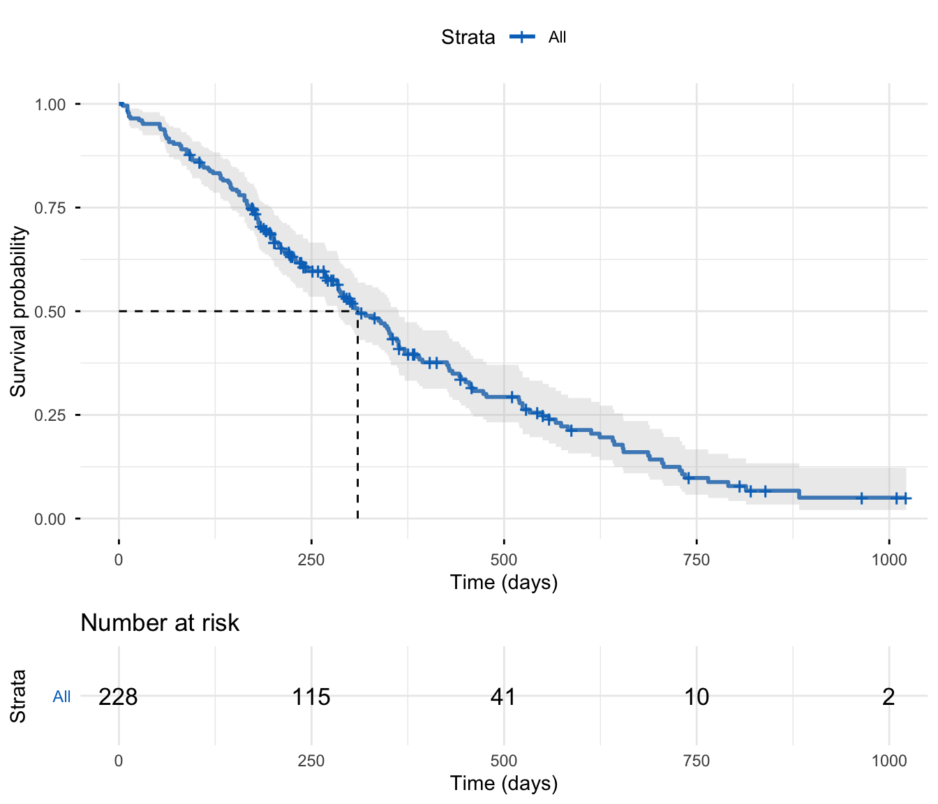
How to read this plot — it is S(t):

• The y-axis is the survival probability S(t); the x-axis is time in days.
• The curve starts at 1.0 at day 0 (everyone alive) and steps down at each death. Each vertical drop is one or more events.
• The small tick marks on the line are censored patients — the moment we lost sight of someone who was still event-free.
• The shaded band is the 95% confidence interval: our uncertainty about the true S(t). Notice it widens at the right, where few patients remain — late estimates are shakier.
• The dashed median line marks where the curve crosses S(t) = 0.5: the median survival is about 310 days for this cohort — half the patients survive beyond ~10 months.
• The number-at-risk table underneath shows how many patients are still being followed (still “at risk”) at each time point — it shrinks as patients die or are censored.

That single picture — built directly from the censored Surv() data, without discarding anyone — is the whole motivation for survival analysis in one image.

Try it live

Draw the overall curve yourself, then split it by sex to preview group comparison — change ~ 1 to ~ sex. The sandbox boots on first Run.

🟢 With an AI agent

Ask Prova “I have follow-up times and an event indicator for my patients — show me how to build a Surv() object and draw a Kaplan-Meier curve in R, and explain what censoring does to my data” — it answers with survival + survminer code you can run on your own data. The runtime is the judge. Ask Prova →

Common issues

You misread censoring as “the event happened.” A censored observation means the event did not occur during follow-up — you only know the subject survived at least that long. In the lung data, status = 1 is censored and status = 2 is the event (death). Treating censored times as event times (or deleting censored patients) biases the curve. Always confirm how your event indicator is coded before you fit anything; with Surv(), a trailing + in the printout is your visual check that censoring is being recognised.

You used a t-test or linear regression on time-to-event data. If your outcome is a duration and some subjects haven’t had the event, ordinary tests don’t apply — they have no way to use the censored subjects honestly. Reach for the survival toolkit instead: Kaplan-Meier to describe, the log-rank test to compare groups, and Cox regression to adjust for covariates.

Frequently asked questions

NoteWhat is survival analysis used for?

Survival analysis answers “how long until an event happens?” It’s used wherever the outcome is a time until an event — time to death or relapse in medical trials, time to a customer churning, time to a part failing in engineering, time to an unemployed person finding a job in economics. Its strength is handling censored subjects, who haven’t had the event by the end of the study.

NoteWhat is censoring in survival analysis?

Censoring means you have incomplete information about a subject’s event time. The most common form, right-censoring, happens when the event hasn’t occurred by the end of follow-up — the subject is still event-free at study close, or was lost to follow-up. You don’t know their exact survival time, only that it is at least as long as the time you observed them. Survival methods are specifically designed to use that partial information rather than discard it.

NoteWhat is the difference between the survival function and the hazard function?

They describe the same data from opposite sides. The survival function S(t) is the probability of surviving past time t (it starts at 1 and falls) — it answers “what fraction are still event-free?” The hazard function h(t) is the instantaneous risk of the event at time t, given survival up to t — it answers “how risky is this moment?” S(t) focuses on not having the event; h(t) focuses on the event occurring. They are mathematically linked, so knowing one determines the other.

NoteWhy can’t I just use logistic or linear regression for time-to-event data?

Because neither handles censoring. Linear regression needs a complete time for every subject, but censored subjects have no observed event time. Logistic regression models a yes/no outcome and ignores when the event happened — and it can’t deal with subjects whose status is “not yet, but maybe later.” Both either delete the censored subjects (biasing the result) or mislabel them. Survival methods use both pieces of information — the follow-up time and whether the event occurred.

NoteWhat is a Kaplan-Meier curve?

The Kaplan-Meier curve is the standard picture of the survival function S(t): a stepped line that starts at 1.0 and drops at each event time, estimated directly from censored data without assuming any particular distribution. Reading it, you can see the proportion surviving at any time, the median survival (where the curve crosses 0.5), and — with a confidence band — how certain the estimate is. It’s almost always the first analysis you run.

Test your understanding

ImportantPractice

1. Run it. In the live cell below, build a Surv() object from the lung data and print the first 10 values. Find an observation with a trailing + — what does it tell you about that patient?
2. Interpret. A Kaplan-Meier curve for a trial shows S(t) crossing 0.5 at 18 months, and S(24 months) = 0.34. In plain words, what is the median survival, and what fraction of patients are alive at 2 years?

NoteHint

A trailing + after a time (e.g. 1010+) marks a censored patient: they were still event-free at that time, so the true survival time is at least that long. For question 2, the median survival is the time where S(t) = 0.5, and S(24 months) = 0.34 reads directly as a percentage alive at 24 months.

NoteSolution

head(Surv(lung$time, lung$status), 10)
#> 306  455  1010+ 210  883  1022+ 310  361  218  166
#> A value like 1010+ is a CENSORED patient: still alive at 1010 days, so their
#> true survival time is at least 1010 days — the event was never observed.

For question 2: the median survival is 18 months (half the patients have had the event by then), and because S(24 months) = 0.34, 34% of patients are still alive at 2 years.

TipQuick check

A patient enrolled in a 2-year trial is still alive and event-free when the study closes at 24 months. How should this patient be recorded in a survival analysis?

NoteShow answer

Right-censored at 24 months. The event (death) was never observed, so we don’t know the patient’s true survival time — only that it is more than 24 months. We keep the patient in the analysis with a follow-up time of 24 months and a censored status; deleting them or recording them as “died at 24 months” would bias the survival estimate.

Conclusion

Survival analysis is the toolkit for time-to-event data — questions of the form “how long until…?”. Its defining feature is censoring: subjects who haven’t had the event by the end of follow-up still carry the information “survived at least this long,” and ordinary methods like the t-test or linear regression have no honest way to use them. Two functions describe the data — the survival function S(t), the probability of surviving past t, and the hazard function h(t), the instantaneous risk at t — and the Kaplan-Meier curve is the picture of S(t), estimated straight from the censored data. With the Surv(time, status) object and a single survfit() call, you drew that picture for the lung-cancer cohort. From here you can estimate it properly, compare it across groups, and model what changes it.

Related lessons

• Kaplan-Meier estimation — estimate the survival curve, medians, and confidence intervals properly. · Log-rank test — compare survival between two or more groups and test the difference. · Cox proportional hazards model — model the effect of covariates on the hazard and report hazard ratios. · Testing the proportional hazards assumption — the diagnostic that keeps a Cox model honest.
• Go further: Survival Analysis — the full series. · Biostatistics — the pillar.

Was this page helpful?

Prove you can do it. Master the whole Survival Analysis in R series — track your path, build projects, and earn a certificate.

Start free →

Go Pro — unlimited Prova on your own data and a verifiable certificate that proves the skill.

from $15/mo billed yearly

Go Pro →

✓ You're Pro — keep going. The runtime is the judge.

Ready to level up?

Try this on your own data with Prova — the runtime is the judge.Open Prova →

Get new R & Python lessons by email

Practical, reproducible, no spam. Unsubscribe anytime.

Double opt-in. We never share your email.

Share this pageXLinkedInRedditHN

Note

Every result on this page was produced by the code shown, run at build time against a pinned R environment — edit any block and Run to reproduce it yourself.