Median Survival Time and 95% Confidence Interval in R

Read the median survival and its 95% CI from a survfit, handle the ‘not reached’ case, and put the medians on the curve with ggsurvplot

Compute the median survival time and its 95% confidence interval in R from a Kaplan-Meier fit with survfit(), read them in plain language, handle the case where the median is “not reached” (NA), get a tidy table with surv_median(), and draw the medians on the survival curve with ggsurvplot(surv.median.line = “hv”) on the NCCTG lung-cancer data.

TipKey takeaways

• Median survival is the time at which half the group has experienced the event — the survival probability \(S(t)\) first drops to 0.5. It is the single most reported number in a survival study.
• Read it straight from a Kaplan-Meier fit: print(survfit(...)) gives the median and its 95% confidence interval per group.
• On the lung-cancer data, median survival is 270 days (95% CI 212–310) for men and 426 days (95% CI 348–550) for women; pooled, it is 310 days (95% CI 285–363).
• surv_median() (survminer) returns the same numbers as a tidy data frame, ready to drop into a table or report.
• When fewer than half the group has the event, the curve never reaches 0.5 and the median is NA (“not reached”) — report a lower quantile, the survival probability at a fixed time, or restricted mean survival time (RMST) instead.
• Put the medians on the curve with ggsurvplot(fit, surv.median.line = "hv").

Introduction

“What’s the typical survival time?” is the first question a clinician, a patient, or a regulator asks of a survival study — and the answer is the median survival time: the point at which half the group has had the event. It is the headline number in oncology trials, the figure that drives labeling claims, and the summary that fits in a single sentence.

You can’t compute it by taking the median of the observed times — censored patients (still alive at last follow-up) would drag it down, because their true survival time is longer than what you saw. The median survival is read off the Kaplan-Meier curve instead: the time at which the estimated survival probability \(S(t)\) first reaches 0.5.

This lesson computes the median survival and its 95% confidence interval in R — from a survfit() fit, with surv_median(), and on the plot — using the classic NCCTG lung-cancer data. You will also handle the case every analyst eventually hits: the median that is “not reached.” If you are new to estimating the curve itself, start with Kaplan-Meier estimation.

The data: the NCCTG lung-cancer study

We use lung, the dataset that ships with the survival package — survival in 228 patients with advanced lung cancer. Load the package and reference lung directly (it auto-attaches with survival, so no data() call is needed):

library(survival)

head(lung[, c("time", "status", "sex")])

  time status sex
1  306      2   1
2  455      2   1
3 1010      1   1
4  210      2   1
5  883      2   1
6 1022      1   1

The three columns we need:

• time — survival (follow-up) time in days.
• status — 1 = censored (alive at last follow-up), 2 = dead (the event).
• sex — 1 = male, 2 = female.

Median survival from survfit()

Fit the Kaplan-Meier curves with survfit(Surv(time, status) ~ group), then print() it. The printout reports the median survival and its 95% confidence interval for each group:

library(survival)

fit <- survfit(Surv(time, status) ~ sex, data = lung)
print(fit)

Call: survfit(formula = Surv(time, status) ~ sex, data = lung)

        n events median 0.95LCL 0.95UCL
sex=1 138    112    270     212     310
sex=2  90     53    426     348     550

Read the median columns:

• median — 270 days for men, 426 days for women. Half the men have died by day 270; half the women, by day 426.
• 0.95LCL / 0.95UCL — the 95% confidence interval for that median: 212–310 days for men, 348–550 days for women.

For the overall median (one curve, no grouping), put 1 on the right-hand side of the formula:

library(survival)

fit_overall <- survfit(Surv(time, status) ~ 1, data = lung)
print(fit_overall)

Call: survfit(formula = Surv(time, status) ~ 1, data = lung)

       n events median 0.95LCL 0.95UCL
[1,] 228    165    310     285     363

Pooled across both sexes, the median survival is 310 days (95% CI 285–363) — between the male (270) and female (426) medians, as expected.

What the median and its CI actually mean

Two phrasings to keep straight:

• The median (270 days for men) is a point estimate: from this sample, our best single guess of the time by which half of men die. It is not “everyone dies at 270 days” and not an average.
• The 95% CI (212–310) is the uncertainty around that estimate. If you repeated the study many times, about 95% of such intervals would contain the true median. The two sexes’ intervals here barely overlap (310 vs 348), which hints at a real difference — but overlapping or non-overlapping CIs are not a formal test. To decide whether survival truly differs, use the log-rank test.

When the median is “not reached”

If fewer than half the patients in a group have the event, the survival curve never drops to 0.5, so the median is undefined. R prints it as NA — often reported as “not reached” (NR). This is common with effective treatments, short follow-up, or heavy censoring.

You can reproduce it with short follow-up: take the female group, but stop watching everyone at day 300 (administrative censoring — anyone still alive then is marked censored). Only 27 of 90 women have died by day 300, so the curve never reaches 0.5:

library(survival)

# Female group with follow-up capped at day 300 (administrative censoring)
women <- subset(lung, sex == 2)
status_300 <- ifelse(women$time > 300, 1, women$status)  # censored if alive past day 300
time_300   <- pmin(women$time, 300)

fit_nr <- survfit(Surv(time_300, status_300) ~ 1)
print(fit_nr)

Call: survfit(formula = Surv(time_300, status_300) ~ 1)

      n events median 0.95LCL 0.95UCL
[1,] 90     27     NA      NA      NA

The median column is NA: with the curve never reaching 0.5, there is no time to report. NA is not zero and not missing data — it usually means good survival (most patients are still event-free). What to report instead:

• A lower quantile — e.g. the time when 25% have died (quantile(fit, probs = 0.25)), which the curve often does reach.
• Survival at a fixed time — “62% event-free at 12 months” via summary(fit, times = 365).
• The lower confidence bound when it exists — “median survival at least X days.”
• Restricted mean survival time (RMST) — the average event-free time up to a chosen horizon; it is always defined even when the median is not (see the note at the end of this lesson).

A tidy median table: surv_median()

print(fit) is fine for reading, but for a report or a table you want the medians as a data frame. survminer’s surv_median() returns exactly that — strata, median, lower, upper:

library(survival)
library(survminer)

fit <- survfit(Surv(time, status) ~ sex, data = lung)
surv_median(fit)

  strata median lower upper
1  sex=1    270   212   310
2  sex=2    426   348   550

Same numbers as the printout — 270 (212–310) for men, 426 (348–550) for women — now in columns you can format or bind into a results table.

Put the medians on the curve: ggsurvplot()

The median is best shown, not just stated. survminer’s ggsurvplot() with surv.median.line = "hv" draws dashed horizontal and vertical guides from \(S(t) = 0.5\) down to each median time — so the reader sees where every curve crosses 50%:

library(survival)
library(survminer)

fit <- survfit(Surv(time, status) ~ sex, data = lung)

ggsurvplot(
  fit,
  data = lung,
  surv.median.line = "hv",  # dashed horizontal + vertical median guides
  conf.int = TRUE,          # 95% confidence bands
  palette = "jco",          # colourblind-safe journal palette
  legend.labs = c("Male", "Female"),
  legend.title = "Sex",
  xlab = "Time (days)",
  ylab = "Survival probability",
  ggtheme = theme_minimal()
)

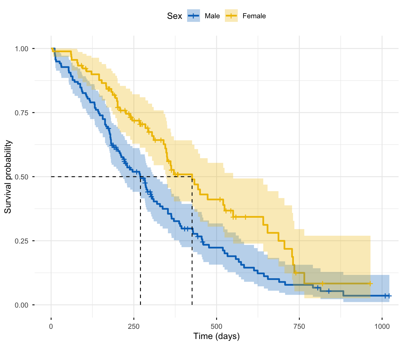
How to read it: the dashed horizontal line sits at 0.5; from where it meets each curve, a dashed vertical line drops to the x-axis — at 270 days (men) and 426 days (women). Those are the medians from survfit(), now visible on the plot. The female curve crosses 0.5 much later, the survival advantage the numbers reported. (For the full publication panel — risk table and log-rank p-value — see Kaplan-Meier estimation.)

Report

Survival was estimated by the Kaplan-Meier method on the NCCTG lung-cancer data (n = 228, 165 deaths). Median overall survival was 310 days (95% CI 285–363). By sex, median survival was 270 days (95% CI 212–310) for men and 426 days (95% CI 348–550) for women.

When a group’s median is not reached, report it explicitly and add a fallback summary:

Median survival was not reached in the treatment arm (vs 280 days, 95% CI 230–340, in the control arm); the 12-month survival probability was 68% (treatment) versus 41% (control).

NoteMedian survival vs RMST

When medians aren’t reached (or survival curves cross / hazards are non-proportional), the restricted mean survival time (RMST) — the average event-free time up to a chosen horizon \(\tau\) — is the standard alternative. Unlike the median, RMST is always defined, and the difference in RMST between arms is a directly interpretable effect (“X extra event-free months on treatment”). See the RMST (restricted mean survival time) lesson (advanced track) for the full workflow.

Which summary when?

TipChoosing your survival summary

• A single headline number, half the group has the event → median survival + its 95% CI (this lesson).
• Fewer than half have the event (median NA) → a lower quantile (e.g. 25th percentile), survival at a fixed time, or RMST.
• An average over a time horizon, or non-proportional hazards / crossing curves → RMST.
• Whether two groups differ → not a CI comparison — the log-rank test.
• An adjusted effect size across covariates → the Cox model (hazard ratio).

Try it live

Read the medians yourself — swap sex for another grouping, change the truncation that triggers a “not reached” median, or pull a different quantile. The sandbox boots on first Run.

🟢 With an AI agent

Ask Prova “compute the median survival with 95% confidence intervals from my Kaplan-Meier fit, tell me what to report when a group’s median is not reached, and draw a ggsurvplot with the median lines” — it answers with survival + survminer code you can run on your own data. The runtime is the judge. Ask Prova →

Common issues

The median is NA (“not reached”). The survival curve never drops to 0.5 because fewer than half the group had the event — so there is no median to report. This is normal with heavy censoring, short follow-up, or genuinely good survival. Don’t read NA as zero or as missing data; report a lower quantile (quantile(fit, probs = 0.25)), the survival probability at a fixed time (summary(fit, times = 365)), or RMST instead.

You compared the two medians and called the difference significant. Two medians (or their confidence intervals) overlapping or not is not a statistical test. Non-overlapping CIs suggest a difference but under- or over-state it; overlapping CIs do not prove “no difference.” To test whether survival differs, run the log-rank test; to quantify the effect, fit a Cox model.

Frequently asked questions

NoteWhat is median survival time?

It is the time at which the estimated survival probability \(S(t)\) first reaches 0.5 — the point by which half the group has experienced the event (e.g. death). It is the most reported single-number summary of a survival curve because it is interpretable (“half the patients survive past X days”) and robust to the long, censored tail that makes a plain mean unreliable.

NoteHow do I calculate median survival in R?

Fit a Kaplan-Meier curve and print it: fit <- survfit(Surv(time, status) ~ group, data); print(fit). The printout reports the median and its 95% confidence interval per group. For a tidy data frame, use survminer’s surv_median(fit). Both read the median straight off the curve — you do not take the median of the raw times (that would mishandle censoring).

NoteWhy is my median survival NA or “not reached”?

Because fewer than half the patients in that group had the event, so the survival curve never drops to 0.5 and the median is undefined. This happens with effective treatments, short follow-up, or heavy censoring — and it is often a good sign. Report a lower quantile (e.g. the 25th percentile), the survival probability at a fixed time, or the restricted mean survival time (RMST) instead.

NoteHow do I interpret the 95% confidence interval for median survival?

It is the range of plausible values for the true median given your sample: if you repeated the study many times, about 95% of such intervals would contain the true median. A wide CI means an imprecise estimate (small group, few events). Comparing two groups’ CIs is not a formal test of difference — use the log-rank test for that.

NoteWhat is the difference between median survival and restricted mean survival time (RMST)?

The median is a single time point (where survival hits 0.5) and is undefined when the curve never gets there. RMST is the average event-free time up to a chosen horizon \(\tau\) (the area under the curve to \(\tau\)) and is always defined. Use the median for a simple headline; use RMST when the median is not reached, the curves cross, or hazards are non-proportional.

Test your understanding

ImportantPractice

1. Run it. In the live cell below, get the median survival and 95% CI for the overall sample (one curve, no grouping) by filling the blank with 1. What is the overall median, and how does it sit relative to the by-sex medians (270 vs 426)?
2. Interpret. A trial reports median survival of NA (“not reached”) in the treatment arm and 280 days in the control arm. In plain words, what does the NA mean, and what should you report instead?

TipHint

For an overall curve with no groups, the right-hand side of the formula is 1. surv_median()’s median column gives the pooled median survival; compare it to the per-sex medians (270 and 426).

TipSolution

fit <- survfit(Surv(time, status) ~ 1, data = lung)
surv_median(fit)
#>   strata median lower upper
#> 1    All    310   285   363

The overall median survival is 310 days (95% CI 285–363) — between the male (270) and female (426) medians, as expected when you pool the two groups.

For question 2: NA (“not reached”) means fewer than half the treatment-arm patients had the event, so the curve never dropped to 0.5 — usually a good sign, not missing data. Don’t report it as zero. Instead report the survival probability at a clinically relevant time (e.g. 12-month survival), a lower quantile, or RMST, and state the lower confidence bound if one exists (“median at least X days”).

TipQuick check

A group’s median survival prints as NA. What does that most likely mean?

NoteShow answer

That more than half the patients in that group were still event-free at the end of follow-up, so the Kaplan-Meier curve never reached a survival probability of 0.5 — the median is undefined (“not reached”), not zero and not a data error. It is often a favourable result. Report a lower quantile, survival at a fixed time, or RMST instead.

Conclusion

You can now report the median survival time in R: fit the curves with survfit(), read the median and its 95% CI from print(fit) or surv_median(), and show the medians on the plot with ggsurvplot(surv.median.line = "hv"). On the lung-cancer data, median survival was 270 days for men, 426 for women, and 310 overall. When fewer than half the group has the event, the median is “not reached” — report a lower quantile, survival at a fixed time, or RMST instead, and remember that comparing medians is not a test: the log-rank test and the Cox model do that.

Related lessons

• Kaplan-Meier estimation — estimate and plot the survival curve the median is read from (the survfit + ggsurvplot workflow in full). · Log-rank test — the formal test of whether two or more survival curves differ (don’t compare medians by eye). · Cox proportional hazards — model survival on one or more covariates and get a hazard ratio per factor.
• Go further: Survival Analysis — the full series. · Biostatistics — the pillar.

Was this page helpful?

Prove you can do it. Master the whole Survival Analysis in R series — track your path, build projects, and earn a certificate.

Start free →

Go Pro — unlimited Prova on your own data and a verifiable certificate that proves the skill.

from $15/mo billed yearly

Go Pro →

✓ You're Pro — keep going. The runtime is the judge.

Ready to level up?

Try this on your own data with Prova — the runtime is the judge.Open Prova →

Get new R & Python lessons by email

Practical, reproducible, no spam. Unsubscribe anytime.

Double opt-in. We never share your email.

Share this pageXLinkedInRedditHN

Note

Every result on this page was produced by the code shown, run at build time against a pinned R environment — edit any block and Run to reproduce it yourself.