Stratified Cox Model in R: Fix a Proportional-Hazards Violation with strata()
When a categorical covariate violates proportional hazards, give it its own baseline hazard with strata() instead of a single hazard ratio — fit, interpret, verify the fix with cox.zph, and visualize with ggadjustedcurves
Biostatistics
Learn the stratified Cox model in R with the survival and survminer packages. When the proportional-hazards assumption fails for a categorical covariate, stratify on it with strata() so each stratum gets its own baseline hazard while the other covariates share common coefficients. Fit the model on the colon-cancer data, interpret why the stratifying variable has no hazard ratio, verify the violation is resolved with cox.zph, compare stratify versus interaction-with-strata, and draw adjusted survival curves with ggadjustedcurves.
Published
June 26, 2026
Modified
July 7, 2026
TipKey takeaways
When a categorical covariate violates proportional hazards (PH), stratify on it. A stratified Cox model gives that variable its own baseline hazard in each stratum, so PH no longer has to hold for it — and the single, misleading hazard ratio is replaced by a per-stratum baseline.
Syntax: wrap the offending variable in strata() — coxph(Surv(time, status) ~ rx + age + strata(differ), data). Everything outside strata() keeps a common coefficient estimated across strata; the stratifying variable gets no hazard ratio.
The tradeoff: you can no longer estimate the stratifying variable’s effect (no HR for it). Stratify a covariate you want to control for, not report — a nuisance confounder or a PH-violator.
Verify the fix: re-run cox.zph() on the stratified model — the violation should disappear.
Stratify vs interaction: stratification assumes the other covariates have the same effect in every stratum. If an effect itself differs across strata, add a covariate * strata() interaction.
Visualize it with survminer’s ggadjustedcurves() — adjusted survival curves, one per stratum.
Introduction
You tested the proportional-hazards assumption of your Cox model, and cox.zph() flagged a covariate: its scaled Schoenfeld residuals drift with time, so its hazard ratio is not constant over follow-up. The single HR the model printed is a misleading time-average. Now what?
You have two honest fixes. If the violator is the treatment or the key effect you want to report, model its time-varying effect — see time-varying covariates. But if the violator is a categorical nuisance covariate — tumor grade, study center, region — that you only need to adjust for, there is a simpler move: stratify on it. Stratification says “let this variable have its own baseline survival in each group, and don’t make me assume PH for it.” You control for it without estimating it.
A classic case: a multi-center trial where center has very different baseline survival (different case-mix, standard of care) and violates PH, but you only care about the treatment effect adjusted for center. Stratify by center, estimate the treatment HR cleanly, and the center’s non-proportionality stops contaminating the result.
This lesson fits a stratified Cox model in R with survival (the model) and survminer (the adjusted-curve plot), on the colon-cancer trial data. You will learn to:
recognize when to stratify (a categorical PH-violator or a nuisance confounder);
write the strata() syntax and read why the stratifying variable loses its hazard ratio;
verify the violation is resolved with cox.zph();
tell stratification apart from a covariate × strata interaction;
and visualize a stratified model with ggadjustedcurves().
NoteWhat stratification changes
A standard Cox model gives every patient the same baseline hazard \(h_0(t)\) and a hazard ratio for each covariate. A stratified Cox model splits the data into strata \(s\) and lets each have its own baseline hazard \(h_{0s}(t)\), while the non-stratified covariates share one set of coefficients:
So the stratifying variable is absorbed into the baseline — it gets no HR (that is the whole point). The other covariates’ HRs are now adjusted within strata: PH must still hold for them, just not for the stratifying variable.
The data: the colon-cancer trial
We use colon, the adjuvant-chemotherapy trial for stage B/C colon cancer that ships with the survival package. It records two outcomes per patient (recurrence and death); we keep the death records (etype == 2), drop the few rows missing key covariates, and label two categorical predictors so the output reads clearly. Build the analysis frame in-block so every example runs standalone:
library(survival)# Death outcome, complete cases on the covariates we modeldcolon <- colon[colon$etype ==2, ]dcolon <- dcolon[!is.na(dcolon$differ) &!is.na(dcolon$nodes), ]# Label the categorical predictors for readable outputdcolon$rx <-factor(dcolon$rx) # treatment armdcolon$differ <-factor(dcolon$differ, labels =c("well", "moderate", "poor")) # tumor gradec(patients =nrow(dcolon), deaths =sum(dcolon$status))
patients   deaths
     888      430
The columns we model:
time / status — survival time in days, and the event indicator (1 = death).
         chisq df       p
rx      2.9292  2 0.23117
age     1.2281  1 0.26777
nodes   0.0137  1 0.90666
extent  3.6014  1 0.05773
differ 16.9031  2 0.00021
GLOBAL 23.7091  7 0.00128
Read the output: the GLOBAL test is significant (p ≈ 0.001), and the culprit is differ (p ≈ 0.0002) — tumor differentiation’s effect on the hazard is not constant over time. Every other covariate is fine (all p > 0.05). So the single hazard ratio the full model reports for differ is misleading, but differ is a prognostic nuisance here — we want to adjust for tumor grade, not publish its HR. That is the textbook signal to stratify on it.
TipStratify, or model the time-varying effect?
The PH-violator is a categorical covariate you only need to control for → stratify it (this lesson). You lose its HR — which you didn’t need.
The PH-violator is the treatment / key effect you must report → model a time-varying coefficient or time interaction (time-varying covariates), so you keep an interpretable early-vs-late effect.
Fit the stratified Cox model with strata()
Move the offending variable inside strata() and leave the rest of the formula unchanged. Each level of differ now gets its own baseline hazard; rx, age, nodes, and extent keep common coefficients estimated across strata:
There is no row for differ. That is not a bug — the stratifying variable is absorbed into three separate baseline hazards (well / moderate / poor), so it has no hazard ratio. You traded its effect estimate for not having to assume PH for it.
rxLev+5FU: HR = 0.68, 95% CI 0.53–0.86, p = 0.0014. Adjusted for the other covariates and stratified by tumor grade, levamisole + fluorouracil cuts the hazard of death by ~32% versus observation — the trial’s key finding, estimated cleanly within grade strata. rxLev alone (HR ≈ 0.91, p = 0.39) shows no convincing benefit.
nodes: HR = 1.09 per positive node, p < 10⁻¹⁸, and extent: HR = 1.65, p < 10⁻⁴ — both strong bad prognostic factors, as expected. age is borderline (HR ≈ 1.01, p = 0.084).
The model is significant overall (likelihood-ratio test p < 0.001), and the number of strata equals the number of differ levels (three).
Verify the fix: cox.zph() on the stratified model
Stratifying should make the violation go away — differ no longer needs to satisfy PH because it’s now a baseline, not a coefficient. Confirm it:
       chisq df    p
rx     2.398  2 0.30
age    1.221  1 0.27
nodes  0.749  1 0.39
extent 2.499  1 0.11
GLOBAL 7.186  5 0.21
The violation is resolved.differ is gone from the test (it’s a baseline now), and the GLOBAL test is non-significant (p ≈ 0.21) — every remaining covariate satisfies proportional hazards. The stratified model is a valid representation of the data; the unstratified one was not. (Stratification slightly lowers the concordance — here ~0.65 vs ~0.66 — because it spends information on three baselines instead of one HR; that is the expected, modest cost of a correct model.)
The signature figure: adjusted survival curves (ggadjustedcurves())
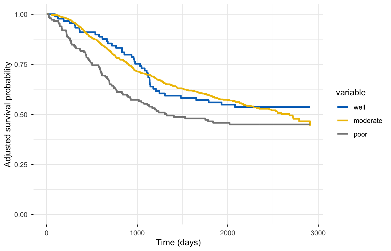
A stratified Cox model has one baseline survival curve per stratum. survminer’s ggadjustedcurves() draws them as adjusted survival curves — the model’s predicted survival for each differ group, holding the other covariates at their average. Pass the fitted model, the data, and the variable to split on:
Read it: each curve is a stratum’s own baseline survival, adjusted for treatment and the other covariates. Well-differentiated tumors survive best (top curve), poorly-differentiated worst (bottom) — and crucially the curves are not constrained to be proportional to each other, which is exactly why stratification handled the PH violation. This is the picture you put in a paper to show how the strata differ.
NoteWhy not ggforest() here?
ggforest() — the forest plot you used for an ordinary Cox model — does not support a model with strata() in the formula (it errors on the missing strata column). For a stratified model, read the hazard ratios from summary() and show the strata with ggadjustedcurves(). If you specifically need a forest plot, fit the non-stratified covariates with the strata as a separate panel, or report the summary() table directly.
Stratify versus interaction: do the other effects differ across strata?
Stratification makes one strong assumption: the non-stratified covariates have the same effect in every stratum (one common rx HR across well / moderate / poor tumors). That is usually what you want — a single, pooled treatment effect adjusted for grade. But what if you suspect the treatment works differently in different grades? Then you need an interaction with the strata, not just stratification.
Add a rx * strata(differ) interaction and compare the two models with a likelihood-ratio test:
library(survival)dcolon <- colon[colon$etype ==2, ]dcolon <- dcolon[!is.na(dcolon$differ) &!is.na(dcolon$nodes), ]dcolon$rx <-factor(dcolon$rx)dcolon$differ <-factor(dcolon$differ, labels =c("well", "moderate", "poor"))# Common treatment effect across strata (what we fit above)fit.strat <-coxph(Surv(time, status) ~ rx + age + nodes + extent +strata(differ),data = dcolon)# Treatment effect ALLOWED to differ across stratafit.inter <-coxph(Surv(time, status) ~ rx *strata(differ) + age + nodes + extent,data = dcolon)anova(fit.strat, fit.inter)
Analysis of Deviance Table
 Cox model: response is  Surv(time, status)
 Model 1: ~ rx + age + nodes + extent + strata(differ)
 Model 2: ~ rx * strata(differ) + age + nodes + extent
   loglik  Chisq Df Pr(>|Chi|)
1 -2381.3
2 -2379.2 4.0634  4     0.3975
Read it: the likelihood-ratio test is non-significant (p ≈ 0.40), so letting the treatment effect vary by tumor grade does not improve the model — the common-effect stratified model is adequate. The treatment benefit is consistent across grades, which is the simpler, more powerful story to report. If this test were significant, you’d keep the interaction and report a per-stratum treatment effect instead of one pooled HR.
TipStratify vs interaction in one line
strata(g) → each stratum its own baseline, but the same covariate effects (one pooled HR).
x * strata(g) → the effect of x is allowed to differ across strata (a separate HR per stratum). Use it only when an LRT (or theory) says the effect genuinely varies.
A second pattern: stratify a nuisance covariate you never wanted an HR for
PH violations aren’t the only reason to stratify. Sometimes you simply want to control for a categorical variable without estimating its effect — a nuisance confounder. Take the lung model from the Cox lesson: suppose sex is a confounder you must adjust for but don’t want to report. Stratify on it and you get the age and ECOG effects adjusted for sex, with no HR for sex:
library(survival)res.cox <-coxph(Surv(time, status) ~ age + ph.ecog +strata(sex), data = lung)summary(res.cox)$coefficients
              coef exp(coef)    se(coef)        z     Pr(>|z|)
age     0.01056625  1.010622 0.009241374 1.143364 2.528875e-01
ph.ecog 0.46242443  1.587919 0.114761098 4.029453 5.590682e-05
age and ph.ecog are estimated within male and female baselines — a clean adjusted estimate without spending a coefficient on sex. (In lung, sex does not actually violate PH — see the PH-testing lesson, where it passed — so here stratifying is a modelling choice to control for a nuisance, not a forced remedy. Both are legitimate uses of strata().)
Report
Because tumor differentiation grade violated the proportional-hazards assumption (cox.zphp < 0.001), we fitted a Cox proportional hazards model stratified by differentiation grade, with treatment arm, age, number of positive nodes, and tumor extent as covariates. Levamisole plus fluorouracil was associated with a significantly lower hazard of death than observation (HR = 0.68, 95% CI 0.53–0.86, p = 0.001), as were fewer positive nodes (HR = 1.09 per node, p < 0.001) and lesser tumor extent (HR = 1.65, p < 0.001). After stratification the proportional-hazards assumption was satisfied for all modelled covariates (GLOBAL cox.zphp = 0.21), and a treatment-by-stratum interaction did not improve the fit (LRT p = 0.40), supporting a common treatment effect across grades.
NoteThe math behind the stratified partial likelihood (optional)
An ordinary Cox model estimates its coefficients from a partial likelihood built over all event times, where each event’s contribution compares the patient who failed to everyone in the risk set at that time. A stratified model builds a separate partial likelihood within each stratum and multiplies them:
\[
L(b) = \prod_{s} L_s(b)
\]
Inside stratum \(s\), the risk set at each event time contains only patients in that stratum, so the stratum’s unspecified baseline hazard \(h_{0s}(t)\)cancels out of every comparison (just as \(h_0(t)\) cancels in the ordinary model). The covariates inside strata() never enter any comparison — patients are only ever compared to others in the same stratum — which is exactly why the stratifying variable gets no coefficient. The non-stratified covariates contribute to all strata’s likelihoods and so share one common estimate \(b\). That single product-of-likelihoods is what coxph() maximizes when you write strata().
Which remedy when?
TipChoosing how to handle a PH violation
A categorical covariate violates PH, and you only need to adjust for it → stratify it (strata()) — this lesson. You lose its HR; you didn’t need it.
The treatment / key effect violates PH → a time-varying coefficient or time interaction (time-varying covariates), so you can report the early-vs-late effect.
The other covariates’ effects differ across strata → a x * strata() interaction (a separate HR per stratum), confirmed by an LRT.
The group survival curves cross (a two-group comparison) → a weighted log-rank test alongside the model.
Try it live
Fit the stratified model yourself — change which variable you stratify on, or swap the dataset. The sandbox boots on first Run.
🟢 With an AI agent
Ask Prova“my Cox model fails the proportional hazards test for a categorical covariate — stratify on it with strata(), show me the new hazard ratios, and confirm cox.zph is now non-significant” — it answers with survival + survminer code you can run on your own data. The runtime is the judge.Ask Prova →
Common issues
You expected a hazard ratio for the stratifying variable and it’s missing. That’s by design, not a bug. A strata() variable is absorbed into a separate baseline hazard per level — it has no HR. If you need to estimate and report that variable’s effect, don’t stratify it: keep it as a covariate and, if it violates PH, model its time-varying effect (time-varying covariates) instead.
Too many strata → thin risk sets and unstable estimates. Each stratum runs its own partial likelihood, so stratifying on a high-cardinality variable (or crossing several with strata(a, b)) can leave strata with few events, inflating standard errors or breaking convergence. Aim for a healthy event count per stratum (a rough rule of thumb: ≥ 10 events each); if strata are sparse, collapse clinically similar levels before stratifying.
You stratified a continuous variable without binning it.strata(age) would create a separate stratum for every distinct age — hundreds of one-patient strata, and a useless model. Stratification is for categorical covariates (or a continuous one cut into a few groups, e.g. strata(cut(age, 3))). A continuous PH-violator usually wants a transformation or a time-varying term, not stratification.
Frequently asked questions
NoteWhat is a stratified Cox model in R?
A stratified Cox model lets a categorical covariate have its own baseline hazard in each group instead of a single hazard ratio. You write it by wrapping the variable in strata(): coxph(Surv(time, status) ~ treatment + age + strata(group), data). The stratifying variable gets no HR (it’s absorbed into the baseline), while the other covariates share common, adjusted coefficients estimated within strata. It’s the standard fix when a categorical covariate violates proportional hazards.
NoteShould I stratify a variable or include it as a covariate?
Include it as a covariate when proportional hazards holds for it and you want to estimate and report its hazard ratio. Stratify it when it violates PH (so a single HR is misleading) or when it’s a nuisance confounder with very different baseline survival across levels that you only need to adjust for, not report. The tradeoff: stratifying buys you robustness to non-proportionality but costs you the effect estimate for that variable.
NoteWhat do I do when the proportional hazards assumption fails?
It depends on which covariate fails. A categorical nuisance covariate → stratify it with strata() (this lesson). The treatment or key effect you must report → model a time-varying coefficient or a time interaction so you can describe the early-vs-late effect (time-varying covariates). For a two-group comparison where the curves cross, a weighted log-rank test is a good companion. Don’t abandon the model — a PH violation is a problem you fix.
NoteWhy does the stratifying variable have no hazard ratio?
Because stratification gives each level its own baseline hazard, and patients are only ever compared to others in the same stratum in the partial likelihood. The stratum’s baseline hazard cancels out of every comparison, so the stratifying variable never enters a coefficient — there is nothing to estimate an HR from. That’s the deliberate tradeoff: you control for the variable without assuming PH for it, but you give up its effect estimate.
NoteWhat’s the difference between stratifying and adding a strata interaction?
Stratifying (strata(g)) gives each group its own baseline but assumes the other covariates have the same effect in every group — one pooled hazard ratio. A strata interaction (x * strata(g)) lets the effect of x itself differ across groups — a separate HR per stratum. Use plain stratification by default; add the interaction only when a likelihood-ratio test (or subject-matter knowledge) shows the effect genuinely varies across strata.
Test your understanding
ImportantPractice
Run it. In the live cell below, fit a Cox model on the colon data without stratifying (rx + age + nodes + extent + differ), then run cox.zph(). Fill the blank. Which covariate violates proportional hazards, and what is the GLOBAL p-value?
Interpret. A reviewer asks why your stratified model reports no hazard ratio for differ. Explain in one or two sentences, and name the one thing you give up by stratifying.
NoteHint
Fill the blank with differ (as a plain covariate, not inside strata()). Read the cox.zph() table: the row with p < 0.05 is the violator, and the GLOBAL row tests the whole model.
NoteSolution
fit <-coxph(Surv(time, status) ~ rx + age + nodes + extent + differ, data = dcolon)cox.zph(fit)#> differ has p ~ 0.0002 (PH violated) and the GLOBAL test p ~ 0.001.#> Every other covariate is non-significant (p > 0.05), so differ is the culprit —#> the signal to stratify on it: strata(differ).
For question 2: the stratifying variable is absorbed into a separate baseline hazard per level, so it never enters a coefficient — there is nothing to compute a hazard ratio from (patients are only compared within strata). What you give up is precisely the effect estimate (HR) for that variable; in exchange you no longer have to assume proportional hazards for it.
TipQuick check
You stratify your Cox model on region (a 5-level categorical confounder that violated PH). After stratifying, cox.zph() GLOBAL is now non-significant (p = 0.40), but there is no hazard ratio for region in the output. Is the model broken?
NoteShow answer
No — that’s exactly what stratification does.region is now five separate baseline hazards, not a coefficient, so it correctly has no HR. The non-significant GLOBAL cox.zph() confirms the violation is resolved and the remaining covariates satisfy proportional hazards. You traded region’s effect estimate (which you didn’t need — it was a nuisance confounder) for a valid model. If you did need region’s effect, you’d model its time-varying effect instead of stratifying.
Conclusion
You can now fix a proportional-hazards violation with a stratified Cox model in R. When cox.zph() flags a categorical covariate you only need to adjust for, wrap it in strata(): each level gets its own baseline hazard, the other covariates keep common adjusted coefficients, and the stratifying variable correctly loses its hazard ratio — the price of not having to assume PH for it. On the colon-cancer data, stratifying by tumor grade resolved the violation (GLOBAL cox.zphp went from 0.001 to 0.21) and gave a clean treatment effect (Lev+5FU HR = 0.68). You verified the fix, told stratification apart from a covariate × strata interaction with a likelihood-ratio test, and drew the adjusted survival curves with ggadjustedcurves(). When the violator is the effect you actually want to report, reach for a time-varying coefficient instead — the next tool in the kit.
Every result on this page was produced by the code shown, run at build time against a pinned R environment — edit any block and Run to reproduce it yourself.