Parametric Survival Models in R: Weibull, AFT, and Extrapolation
Assume a distribution for survival time with survreg and flexsurv — fit Weibull, exponential, log-normal and log-logistic models, interpret the time ratio, choose by AIC, convert AFT to a hazard ratio, and extrapolate beyond follow-up
Biostatistics
Learn parametric survival models in R with the survival and flexsurv packages. Fit Weibull, exponential, log-normal and log-logistic accelerated failure time (AFT) models with survreg(), interpret the time ratio (not the hazard ratio), choose a distribution by AIC, overlay the fitted curve on the Kaplan-Meier, convert a Weibull AFT to a Cox-style hazard ratio, fit a flexible Royston-Parmar spline model with flexsurvspline(), and extrapolate survival beyond the observed follow-up for health-economic models.
Published
June 26, 2026
Modified
July 7, 2026
TipKey takeaways
A parametric survival model assumes survival time follows a known distribution (Weibull, exponential, log-normal, log-logistic). In exchange for that assumption you get a smooth survival and hazard curve, full distributional summaries (any quantile, the mean), and — the headline feature — extrapolation beyond the observed follow-up.
Most parametric models are accelerated failure time (AFT) models: covariates stretch or shrink the survival timeline. The effect size is a time ratio, not a hazard ratio — “being female multiplies survival time by ~1.49” rather than “cuts the hazard by 41%”.
Fit them with survreg(Surv(time, status) ~ ., dist = "weibull") (the survival package) or flexsurv::flexsurvreg() (nicer summaries, built-in plotting, more distributions).
Choose the distribution by AIC and by overlaying the fitted curve on the Kaplan-Meier — the lowest AIC that also tracks the KM curve wins. On the lung data the Weibull fits best (AIC 2275).
The Weibull is special: it is both AFT and proportional hazards, so you can convert its time ratio to a Cox-style hazard ratio — they agree (HR ≈ 0.58 for sex, same as the Cox model).
When a standard distribution is too rigid, fit a flexible spline model with flexsurvspline() (Royston-Parmar) for an arbitrary hazard shape.
Introduction
Your trial followed patients for two years and the Cox model gave you clean hazard ratios. Now the health-economics team needs the 5-year survival for a cost-effectiveness model — a number your data never observed. The Cox model can’t give it to you: it leaves the baseline hazard unspecified, so it has nothing to say beyond the last event time. You need a model that assumes a shape for the whole survival curve, so it can be extrapolated.
That is a parametric survival model. Instead of leaving the baseline hazard free (the Cox model’s trade-off), you assume survival time follows a specific distribution — Weibull, exponential, log-normal, log-logistic — and estimate its parameters. The payoff:
a smooth survival and hazard curve (no step function), and any quantile or the mean, not just the median;
extrapolation of survival beyond the observed follow-up — the reason health-economic and cost-effectiveness models nearly always use a parametric fit;
a covariate effect expressed as a time ratio (the accelerated failure time interpretation), which many people find more intuitive than a hazard ratio.
This lesson fits the parametric family in R with survival’s survreg() and the more capable flexsurv, choosing a distribution by AIC and a fitted-vs-Kaplan-Meier overlay, on the same NCCTG lung-cancer data used throughout this series so you can reproduce every number.
NoteAFT vs PH — two ways to model a covariate
A proportional hazards (PH) model (Cox) says a covariate multiplies the hazard by a constant — the hazard ratio.
An accelerated failure time (AFT) model says a covariate multiplies survival time by a constant — the time ratio. A time ratio of 1.5 means the covariate stretches the survival timeline by 50% (longer survival); below 1 means it accelerates failure (shorter survival).
The Weibull distribution is the one model that is both AFT and PH, so its time ratio converts cleanly to a hazard ratio. The exponential is too (it is Weibull with a constant hazard); log-normal and log-logistic are AFT only.
The data and the question
We use lung, the North Central Cancer Treatment Group dataset that ships with the survival package (228 advanced lung-cancer patients). The coding is the survival-package standard: status is 1 = censored / 2 = dead, sex is 1 = male / 2 = female, ph.ecog is the ECOG performance score. We model survival on sex, age, and ECOG score — the same covariates as the Cox lesson, so you can compare the two frameworks directly.
The Surv(time, status) object is the response, exactly as in the Cox model — the parametric models just make a different assumption about what generated those times.
Fit a Weibull AFT model with survreg()
Start with the workhorse, the Weibull model. survreg() (survival package) fits parametric AFT models; pick the distribution with dist. The Surv(time, status) response goes on the left, the covariates on the right:
library(survival)fit.wb <-survreg(Surv(time, status) ~ sex + age + ph.ecog, data = lung, dist ="weibull")summary(fit.wb)
Call:
survreg(formula = Surv(time, status) ~ sex + age + ph.ecog, data = lung,
    dist = "weibull")
               Value Std. Error     z       p
(Intercept)  6.27344    0.45358 13.83 < 2e-16
sex          0.40109    0.12373  3.24  0.0012
age         -0.00748    0.00676 -1.11  0.2690
ph.ecog     -0.33964    0.08348 -4.07 4.7e-05
Log(scale)  -0.31319    0.06135 -5.11 3.3e-07

Scale= 0.731

Weibull distribution
Loglik(model)= -1132.4   Loglik(intercept only)= -1147.4
    Chisq= 29.98 on 3 degrees of freedom, p= 1.4e-06
Number of Newton-Raphson Iterations: 5
n=227 (1 observation effacée parce que manquante)
Read the output — and mind the parameterization.survreg() works on the log-time scale, so its coefficients are AFT coefficients, not log-hazard ratios:
sex = 0.401. A positive coefficient means the covariate lengthens survival time. Exponentiate to get the time ratio: exp(0.401) ≈ 1.49. Being female (sex 2 vs 1) multiplies survival time by about 1.49 — women survive roughly 49% longer, holding age and ECOG fixed.
ph.ecog = −0.340. A negative coefficient shortens survival. exp(−0.340) ≈ 0.71: each one-point worsening of the ECOG score multiplies survival time by 0.71 (a 29% shorter timeline) — a bad prognostic factor, as before.
age = −0.0075, p = 0.27. Time ratio ≈ 0.99 and not significant — age drops out after adjustment, the same story the Cox model told.
Log(scale) = −0.313 → Scale = 0.731. This is the Weibull scale in survreg’s parameterization; its reciprocal is the Weibull shape, 1 / 0.731 ≈ 1.37. A shape > 1 means the hazard increases over time (risk of death rises as the disease progresses); shape = 1 would be a constant hazard (the exponential); shape < 1 a falling hazard.
The model is significant — the likelihood-ratio χ²(3) = 29.98, p = 1.4×10⁻⁶, soundly beating the intercept-only null.
NoteThe sign trap (AFT coefficients run opposite to PH)
In an AFT model a positive coefficient is good (longer survival); in a PH/Cox model a positive coefficient is bad (higher hazard). Same protective effect of sex, opposite sign: AFT sex = +0.40 (stretches time), Cox sex = −0.53 (lowers hazard). Always know which framework your software is reporting before you read a sign.
Fit the whole family and choose by AIC
No single distribution is right a priori — fit several and compare. Fit the exponential, Weibull, log-normal, and log-logistic models, then rank them by AIC (lower = better fit, penalized for parameters):
library(survival)f <-Surv(time, status) ~ sex + age + ph.ecogfits <-list(exponential =survreg(f, data = lung, dist ="exponential"),weibull =survreg(f, data = lung, dist ="weibull"),lognormal =survreg(f, data = lung, dist ="lognormal"),loglogistic =survreg(f, data = lung, dist ="loglogistic"))aic <-sapply(fits, AIC)tab <-data.frame(distribution =names(aic), AIC =round(aic, 1))tab <- tab[order(tab$AIC), ]tab$delta_AIC <-round(tab$AIC -min(tab$AIC), 1)tab
Read it: the Weibull has the lowest AIC (2274.9), with log-logistic a close second (ΔAIC ≈ 10) and the exponential clearly worse (ΔAIC ≈ 20) — its constant-hazard assumption is too rigid for these data, where risk rises over time (recall the Weibull shape ≈ 1.37). A rule of thumb: ΔAIC < 2 = indistinguishable, 4–7 = clearly worse, > 10 = essentially no support. Here the choice is the Weibull.
WarningAIC alone is not enough — always look at the curve
AIC ranks the candidates relative to each other, but it can’t tell you whether the best one actually fits. Two distributions with similar AIC can extrapolate to wildly different long-term survival. Always pair the AIC table with the fitted-vs-Kaplan-Meier overlay below (does the curve track the data?) — and, for an extrapolation, sanity-check the long-tail shape against clinical knowledge.
The signature check: fitted curves overlaid on the Kaplan-Meier
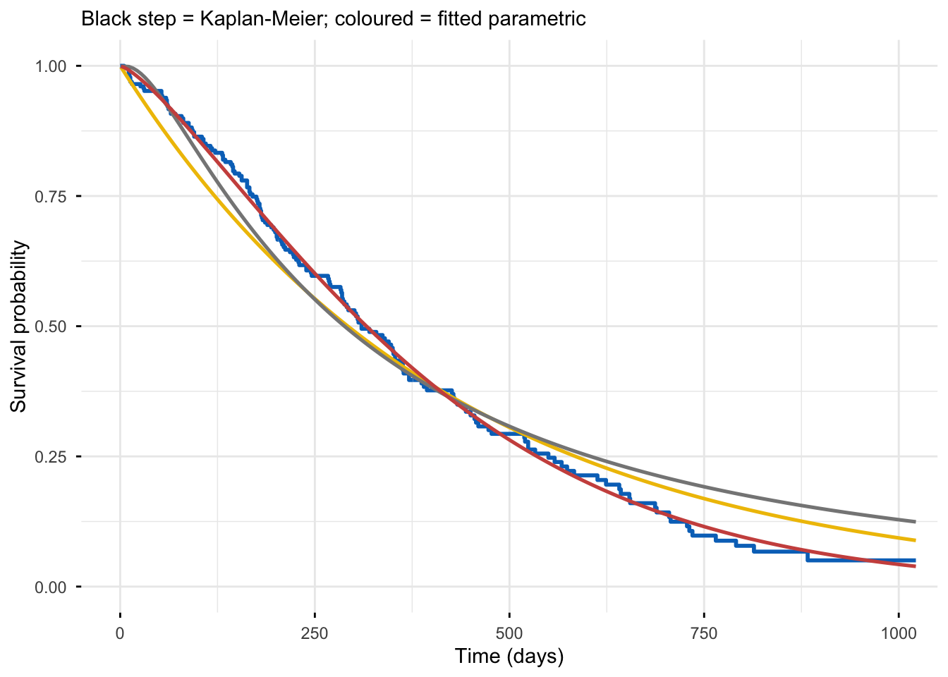
The decisive diagnostic is visual: overlay each fitted parametric survival curve on the Kaplan-Meier estimate (the non-parametric truth). A good distribution hugs the KM step function; a bad one drifts away. We build the curves from intercept-only fits (the marginal survival), then plot them over the KM with survminer’s ggsurvplot():
library(survival)library(survminer)# Non-parametric Kaplan-Meier (the reference)km <-survfit(Surv(time, status) ~1, data = lung)# A grid of times to evaluate the fitted curves ont <-seq(1, max(lung$time), length.out =200)# Marginal (intercept-only) parametric fits, predicted survival at each tpred <-function(dist) { m <-survreg(Surv(time, status) ~1, data = lung, dist = dist)# survreg gives quantiles; invert to S(t) on the time grid (row 1 = the marginal fit) q <-seq(0.001, 0.999, by =0.001) pt <-predict(m, type ="quantile", p = q)[1, ]approx(pt, 1- q, xout = t, rule =2)$y}curves <-data.frame(time =rep(t, 3),surv =c(pred("weibull"), pred("exponential"), pred("lognormal")),dist =rep(c("Weibull", "Exponential", "Log-normal"), each =length(t)))ggsurvplot(km, data = lung, conf.int =FALSE, censor =FALSE,palette ="black", legend ="none",ggtheme =theme_minimal(),xlab ="Time (days)", ylab ="Survival probability")$plot +geom_line(data = curves, aes(x = time, y = surv, colour = dist), linewidth =0.9) + ggsci::scale_color_jco(name ="Fitted") +labs(subtitle ="Black step = Kaplan-Meier; coloured = fitted parametric")
Read it: the Weibull (its shape lets the hazard rise over time) tracks the KM curve closely from start to finish — confirming the AIC verdict visually. The log-normal is close but rides slightly high in the tail. The exponential clearly fails: its constant-hazard assumption forces a curve that sits above the data early and falls too slowly — exactly the kind of mismatch AIC flagged. The picture and the AIC table agree: trust the Weibull.
flexsurv: cleaner summaries, the same Weibull
The flexsurv package fits the same models with a friendlier interface, direct survival/hazard prediction, confidence intervals on every quantity, and built-in plotting. Its flexsurvreg() reports the Weibull on its natural scale (shape and scale directly) plus the covariate effects as time ratios in the exp(est) column — no manual exponentiation:
library(survival)library(flexsurv)fs.wb <-flexsurvreg(Surv(time, status) ~ sex + age + ph.ecog, data = lung, dist ="weibull")fs.wb
Call:
flexsurvreg(formula = Surv(time, status) ~ sex + age + ph.ecog,
    data = lung, dist = "weibull")

Estimates:
         data mean  est        L95%       U95%       se         exp(est)
shape           NA   1.37e+00   1.21e+00   1.54e+00   8.39e-02         NA
scale           NA   5.30e+02   2.18e+02   1.29e+03   2.41e+02         NA
sex       1.40e+00   4.01e-01   1.59e-01   6.44e-01   1.24e-01   1.49e+00
age       6.25e+01  -7.48e-03  -2.07e-02   5.78e-03   6.76e-03   9.93e-01
ph.ecog   9.52e-01  -3.40e-01  -5.03e-01  -1.76e-01   8.35e-02   7.12e-01
         L95%       U95%
shape           NA         NA
scale           NA         NA
sex       1.17e+00   1.90e+00
age       9.79e-01   1.01e+00
ph.ecog   6.05e-01   8.39e-01

N = 227,  Events: 164,  Censored: 63
Total time at risk: 69522
Log-likelihood = -1132.439, df = 5
AIC = 2274.877
Read it: flexsurv reports shape ≈ 1.37 and the covariate time ratios in the exp(est) column directly — sex 1.49 (95% CI 1.17–1.90), ph.ecog 0.71 (0.60–0.84), age 0.99 (ns) — identical to what we computed by hand from survreg() (the log-likelihood, −1132.4, and AIC, 2274.9, match exactly: it is the same model, a nicer printout). For everyday parametric work flexsurv is the more convenient engine; survreg() is the base-survival workhorse worth knowing because it is everywhere.
Convert the Weibull AFT to a hazard ratio
Because the Weibull is both AFT and PH, you can turn its time ratio into a Cox-style hazard ratio — useful when a journal or a colleague expects HRs. The conversion uses the Weibull shape p:
The Weibull-implied hazard ratio for sex is ≈ 0.58 — being female cuts the hazard by ~42% — which matches the Cox model’s HR of 0.58 from the Cox lesson almost exactly. Two frameworks, two effect sizes (a time ratio of 1.49 and a hazard ratio of 0.58), telling the same story about the same protective effect.
The headline feature: extrapolate beyond follow-up
This is what a parametric model gives you that Cox cannot. Once the distribution is fixed, the survival curve is defined for all time — so you can read off survival at horizons your data never reached, and full distributional summaries. Use flexsurv’s summary() with type = "survival" (with confidence intervals) or type = "mean":
library(survival)library(flexsurv)fs.wb <-flexsurvreg(Surv(time, status) ~ sex + age + ph.ecog, data = lung, dist ="weibull")# A typical male vs female patient (mean age, ECOG = 1)nd <-data.frame(sex =c(1, 2), age =mean(lung$age, na.rm =TRUE), ph.ecog =1)# Predicted survival at 1 and 2 years (730 days is past most follow-up)summary(fs.wb, newdata = nd, t =c(365, 730), type ="survival", tidy =TRUE)
  time        est        lcl       ucl sex      age ph.ecog
1  365 0.35186771 0.28750912 0.4195064   1 62.44737       1
2  730 0.06750298 0.03781955 0.1118319   1 62.44737       1
3  365 0.54691334 0.45547836 0.6333649   2 62.44737       1
4  730 0.21068601 0.12134108 0.3111966   2 62.44737       1
The model predicts 1-year survival of 35% for a typical male vs 55% for a female, and 2-year survival of 7% vs 21% — even though relatively few patients were followed a full two years. Each prediction comes with a confidence interval (lcl/ucl); the band widens the further you extrapolate, an honest signal of growing uncertainty. You can also read the mean survival time directly (the area under the curve, undefined for a KM curve that never reaches zero):
library(survival)library(flexsurv)fs.wb <-flexsurvreg(Surv(time, status) ~ sex + age + ph.ecog, data = lung, dist ="weibull")nd <-data.frame(sex =c(1, 2), age =mean(lung$age, na.rm =TRUE), ph.ecog =1)summary(fs.wb, newdata = nd, type ="mean", tidy =TRUE)
       est      lcl      ucl sex      age ph.ecog
1 323.4767 283.2366 374.2865   1 62.44737       1
2 483.0970 397.7197 587.3424   2 62.44737       1
Mean survival ≈ 323 days for a male vs 483 days for a female — and 483 / 323 ≈ 1.49, the time ratio again. That mean survival time, multiplied by a utility weight and discounted, is exactly the input a cost-effectiveness model needs.
WarningExtrapolation is a privilege, not a free lunch
The survival curve beyond your data is entirely an assumption — it is the distribution’s shape, not evidence. A Weibull and a log-normal that fit the observed data almost equally well can predict very different 5-year survival. Always (1) compare extrapolations across the plausible distributions, (2) widen the horizon only as far as the shape is clinically defensible, and (3) validate against external data (registries, longer studies) where you can. Report the long-tail uncertainty, don’t hide it.
When a standard distribution is too rigid: flexible splines
Sometimes none of the named distributions captures the hazard shape — it might rise, plateau, then fall. Royston-Parmar flexible parametric (spline) models model the log-cumulative-hazard as a natural cubic spline in log-time, so the hazard can take almost any smooth shape while keeping the extrapolation and prediction machinery. Fit one with flexsurvspline(), choosing the number of internal knots k:
library(survival)library(flexsurv)fs.sp <-flexsurvspline(Surv(time, status) ~ sex + age + ph.ecog,data = lung, k =2, scale ="hazard")# Compare the spline's fit to the Weibull by AICfs.wb <-flexsurvreg(Surv(time, status) ~ sex + age + ph.ecog, data = lung, dist ="weibull")c(weibull_AIC =AIC(fs.wb), spline_AIC =AIC(fs.sp))
weibull_AIC  spline_AIC
   2274.877    2277.403
Here the spline’s AIC (≈ 2277) is slightly higher than the Weibull’s (≈ 2275): the extra flexibility isn’t needed for the lung data — the Weibull’s smooth, monotonically rising hazard already fits. That is the right outcome to see: reach for a spline when a named distribution visibly fails the KM overlay, not by default. When you do need it, flexsurvspline() gives you a flexible hazard shape without giving up extrapolation — and plot(fs.sp) overlays its fitted curve on the KM for the same visual check.
Report
Survival was modelled with a parametric accelerated failure time (AFT) model on the NCCTG lung-cancer data (n = 227, 164 deaths). Four distributions were compared by AIC; the Weibull fitted best (AIC = 2274.9, shape = 1.37, indicating a hazard that increases over time) and tracked the Kaplan-Meier estimate closely. Female sex was associated with longer survival (time ratio = 1.49, 95% CI 1.17–1.90; equivalent hazard ratio = 0.58, matching the Cox model), as was a lower ECOG performance score (time ratio = 0.71 per one-point worsening, 95% CI 0.60–0.84); age was not significant. The fitted model estimated a 2-year survival of 21% for a typical female versus 7% for a male patient (mean age, ECOG = 1).
NoteThe math behind AFT and the Weibull duality (optional)
An accelerated failure time model writes log survival time as a linear function of covariates plus an error term:
\[
\log T = \mu + \gamma_1 x_1 + \dots + \gamma_p x_p + \sigma \, W
\]
where \(W\) is a standard error distribution (its choice — extreme-value, normal, logistic — sets the survival distribution: Weibull, log-normal, log-logistic). A covariate shifts log-time by \(\gamma_j\), so it multiplies time by \(e^{\gamma_j}\) — the time ratio. This is why a positive \(\gamma\) lengthens survival.
The Weibull is the one distribution that is both AFT and proportional hazards. Its hazard is \(h(t) = p\,\lambda\,t^{\,p-1}\) with shape \(p\) and scale \(\lambda\). Writing the covariate effect through \(\lambda\) gives a constant hazard ratio; writing it through the timeline gives a time ratio. The two parameterizations are linked by the shape:
So the AFT coefficient \(\gamma_j\) from survreg() and the PH coefficient from coxph() differ only by the factor \(-p\) — and on the lung data both yield HR ≈ 0.58 for sex. The exponential is the special case \(p = 1\) (constant hazard); log-normal and log-logistic are AFT but not PH, so they have a time ratio but no single hazard ratio.
Which model when?
TipCox vs parametric — pick by what you need
A hazard ratio with no distributional assumption, primary efficacy analysis → Cox proportional hazards (semi-parametric, the default).
Extrapolation beyond follow-up, mean survival, health-economic / cost-effectiveness inputs → a parametric model (this lesson) — Cox simply cannot extrapolate.
A time-ratio interpretation (“treatment extends survival by 40%”), or PH is violated so the single HR is misleading → an AFT model (Weibull / log-normal / log-logistic).
None of the named shapes fits the hazard → a flexible spline model (flexsurvspline).
Unsure which distribution → fit several, rank by AIC, and confirm with the Kaplan-Meier overlay.
Try it live
Fit the parametric family yourself — change the distribution, swap covariates, or read off survival at a new time horizon. The sandbox boots on first Run.
🟢 With an AI agent
Ask Prova“fit a Weibull parametric survival model on my data, give me the time ratios and the equivalent hazard ratios, choose the best distribution by AIC, and extrapolate survival to 5 years” — it answers with survival + flexsurv code you can run on your own data. The runtime is the judge.Ask Prova →
Common issues
You read the AFT coefficient as a hazard ratio.survreg() works on the log-time scale: a positive coefficient means longer survival (a good effect), and exp(coef) is a time ratio, not a hazard ratio. This is the opposite sign convention to coxph(). If you need an HR from a Weibull fit, convert it explicitly — HR = exp(-coef * shape) with shape = 1 / fit$scale — don’t exponentiate the AFT coefficient and call it an HR.
You picked a distribution by AIC alone and the extrapolation is nonsense. AIC ranks the candidates against each other on the observed data; it says nothing about the unobserved tail. Two distributions with near-identical AIC can predict very different 5-year survival. Always overlay the fitted curve on the Kaplan-Meier and sanity-check the long-tail shape against clinical knowledge before trusting an extrapolation.
You extrapolated far past the data and reported a point estimate as if it were certain. The survival curve beyond follow-up is the distribution’s assumption, not evidence — the confidence band widens for a reason. Compare extrapolations across the plausible distributions, report the range, and validate against external data where possible. A single confident 10-year survival number from 2 years of data is a red flag.
Frequently asked questions
NoteAFT vs Cox / proportional hazards — which should I use?
Use Cox when you want a hazard ratio with no distributional assumption and don’t need to predict beyond your data — it is the default for primary efficacy analysis. Use a parametric / AFT model when you need to extrapolate survival beyond follow-up (health economics, lifetime cost-effectiveness), want the mean survival time or any quantile, prefer a time-ratio interpretation, or the proportional-hazards assumption is violated. Many analyses use Cox for the primary estimate and a parametric model for the extrapolation.
NoteHow do I get a hazard ratio from a Weibull model?
The Weibull is both AFT and proportional hazards, so its AFT coefficient converts to a hazard ratio with the shape parameter p: HR = exp(-coef * p), where coef is the survreg() coefficient and p = 1 / fit$scale. Equivalently HR = (time ratio)^(-p). On the lung data this gives HR ≈ 0.58 for sex, matching the Cox model. This conversion works only for the Weibull and exponential — log-normal and log-logistic are AFT but not PH, so they have a time ratio but no single hazard ratio.
NoteWhat does the time ratio mean in an AFT model?
A time ratio is the factor by which a covariate multiplies survival time. A time ratio of 1.49 for female sex means women’s survival timeline is stretched by ~49% (longer survival); a time ratio below 1 means the covariate accelerates failure (shorter survival). It is the AFT analogue of the hazard ratio: the hazard ratio multiplies the risk, the time ratio multiplies the time.
NoteHow do I choose between Weibull, exponential, log-normal and log-logistic?
Fit all the candidates and rank them by AIC (lower is better) — then confirm the winner by overlaying its fitted survival curve on the Kaplan-Meier. The exponential assumes a constant hazard, so it usually loses when risk changes over time; the Weibull (an increasing or decreasing hazard) is the common default. A ΔAIC below 2 means two models are indistinguishable; above 10 means essentially no support. Never trust AIC alone for an extrapolation — check the curve and the clinical plausibility of the tail.
NoteWhat is survreg vs flexsurv — which package should I use?
survreg() (survival package) is the base-R workhorse: it fits AFT models on the log-time scale and is everywhere, but you exponentiate coefficients yourself and it covers fewer distributions. flexsurvreg() (flexsurv package) reports parameters on their natural scale, gives time ratios directly with confidence intervals, predicts survival/hazard/mean at any time, and adds distributions plus flexsurvspline() for flexible shapes. Use survreg() for a quick base-survival fit; use flexsurv for serious parametric work, prediction, and extrapolation.
Test your understanding
ImportantPractice
Run it. In the live cell below, fit a parametric model with the log-logistic distribution instead of the Weibull (fill the blank), then compare its AIC to the Weibull’s. Which distribution does AIC prefer on these data?
Interpret. An AFT model reports a treatment coefficient of 0.30 (survreg, Weibull, shape = 1.2). In plain words, what is the time ratio, and — converting — the equivalent hazard ratio?
NoteHint
Fill the blank with "loglogistic". Compare the two AIC values — the lower one is the better fit. Recall from the AIC table that the Weibull had the lowest AIC of the four candidates, with log-logistic a few points behind.
NoteSolution
fit.ll <-survreg(Surv(time, status) ~ sex + age + ph.ecog, data = lung, dist ="loglogistic")fit.wb <-survreg(Surv(time, status) ~ sex + age + ph.ecog, data = lung, dist ="weibull")c(loglogistic_AIC =AIC(fit.ll), weibull_AIC =AIC(fit.wb))#> loglogistic_AIC ~ 2285, weibull_AIC ~ 2275 — the WEIBULL is preferred (lower AIC, ΔAIC ~ 10).
For question 2: the time ratio is exp(0.30) ≈ 1.35 — treatment multiplies survival time by about 1.35 (35% longer survival). Converting to a hazard ratio with the shape: HR = exp(-0.30 * 1.2) ≈ 0.70 — a 30% lower hazard of the event. Both describe the same beneficial treatment effect, one as longer time, one as lower risk.
TipQuick check
A parametric survival model reports a time ratio of 0.65 for a covariate. What does it mean for survival?
NoteShow answer
Shorter survival — a harmful covariate. A time ratio below 1 means the covariate multiplies survival time by less than 1 (here by 0.65), so it shrinks the survival timeline — it accelerates failure. The equivalent hazard ratio would be above 1 (higher risk). A time ratio above 1 would mean longer survival (a protective factor).
Conclusion
You can now fit and interpret parametric survival models in R. Fit the AFT family with survreg() or flexsurv::flexsurvreg(), read the covariate effect as a time ratio (mind the log-time sign convention), choose a distribution by AIC and the Kaplan-Meier overlay, and — because the Weibull is both AFT and PH — convert its time ratio to a hazard ratio that matches the Cox model. The payoff that Cox can’t offer is extrapolation: smooth survival curves, mean survival, and survival at any horizon, the inputs a health-economic model lives on. When no named distribution fits the hazard shape, a flexsurvspline() flexible model handles it. The one discipline to carry forward: an extrapolation is an assumption, so always check the fit, compare distributions, and report the uncertainty in the tail.
Every result on this page was produced by the code shown, run at build time against a pinned R environment — edit any block and Run to reproduce it yourself.