Competing Risks Analysis in R: Cumulative Incidence and Fine-Gray

When a patient can fail from more than one cause, naive Kaplan-Meier overstates the risk — estimate the cumulative incidence function with tidycmprsk, test it with Gray’s test, and model it with cause-specific and Fine-Gray regression

Run a competing risks analysis in R with the survival and tidycmprsk packages. See why 1 - Kaplan-Meier overestimates the cumulative incidence of an event when a competing event (such as death) can occur first, estimate the cumulative incidence function (CIF) with cuminc and plot it with ggsurvfit’s ggcuminc, compare groups with Gray’s test, and choose between a cause-specific Cox model and a Fine-Gray subdistribution hazard model — on the survival package’s mgus2 dataset.

TipKey takeaways

• Competing risks arise when a patient can fail from more than one cause and one event prevents observing another — most often, death before the event of interest (e.g. disease progression). A competing event is not ordinary censoring: a censored patient could still go on to have the event, a patient who died never can.
• Treating a competing event as censoring and reading 1 − Kaplan-Meier as the incidence overstates the risk. On the mgus2 data, the naive curve puts the 20-year incidence of progression at ~21%, while the correct cumulative incidence function (CIF) puts it at ~10% — the gap is the bias.
• The right summary is the cumulative incidence function: estimate it with tidycmprsk::cuminc(Surv(time, event) ~ group), plot it with ggsurvfit::ggcuminc(), and compare groups with Gray’s test (printed by cuminc()).
• Two regression models answer two different questions: the cause-specific Cox model (censor the competitor) is for etiology (“does this covariate drive the event rate?”); the Fine-Gray subdistribution model crr() is for prediction (“does this covariate change the cumulative incidence?”). They can disagree — and that’s informative, not a bug.
• The event variable must be a factor whose first level is the censoring code — get the coding right and the whole analysis follows.

Introduction

Picture an oncology trial in an older population. You want time to disease progression, but many patients die of something else first — a heart attack, an infection, a second cancer. A patient who dies can never progress: death has removed them from the population that could still have the event you care about.

This is a competing risk, and it breaks the standard survival toolkit. The Kaplan-Meier estimator and the Cox model assume that a patient who leaves your view is censored — that they could still have the event if you kept following them. That is true for a patient who simply reached the end of the study. It is false for a patient who died: they are gone for good. Censor the deaths and pretend they might still progress, and you overestimate how many patients will progress.

This lesson does competing risks the right way with survival and tidycmprsk, using the mgus2 dataset — a textbook competing-risks problem where patients with monoclonal gammopathy can either progress to a plasma-cell malignancy or die first.

NoteCompeting event vs censoring — the one distinction to get right

A patient leaves the risk set for one of two reasons:

• Censoring — we stopped watching (study ended, lost to follow-up). They could still have the event. Standard survival analysis handles this.
• Competing event — a different event happened that makes the event of interest impossible (death before progression). They can never have it now.

Treat a competing event as censoring and you assume the impossible — that a dead patient might still progress. That single mistake is what inflates the risk.

The data: progression vs death in mgus2

We use mgus2, which ships with the survival package: 1384 patients with monoclonal gammopathy of undetermined significance (MGUS), followed for decades. Two things can happen:

• Progression to a plasma-cell malignancy (PCM) — the event of interest — recorded by pstat (1 = progressed) at time ptime (months).
• Death — the competing event — recorded by death (1 = died) at time futime (months).

library(survival)

head(mgus2[, c("id", "age", "sex", "ptime", "pstat", "futime", "death")])

  id age sex ptime pstat futime death
1  1  88   F    30     0     30     1
2  2  78   F    25     0     25     1
3  3  94   M    46     0     46     1
4  4  68   M    92     0     92     1
5  5  90   F     8     0      8     1
6  6  90   M     4     0      4     1

Build the single competing-risks event variable

Competing risks needs one time and one event variable with a code for each outcome. The rule: if a patient progressed, use the progression time and code it as the event; otherwise use the follow-up time and code it as death or censoring. tidycmprsk requires the event to be a factor whose first level is the censoring code — everything downstream depends on this.

library(survival)

mg <- mgus2
# One event time: progression time if progressed, else follow-up time
mg$etime <- ifelse(mg$pstat == 1, mg$ptime, mg$futime)

# One event code: 0 = censored, 1 = progression (PCM), 2 = death
ecode <- with(mg, ifelse(pstat == 1, 1, ifelse(death == 1, 2, 0)))

# Factor with the CENSOR level FIRST (tidycmprsk requirement)
mg$event <- factor(ecode, levels = c(0, 1, 2),
                   labels = c("censor", "pcm", "death"))

table(mg$event)

censor    pcm  death 
   409    115    860 

So 115 patients progressed, 860 died first (the competing event), and 409 were censored. With deaths outnumbering progressions roughly 7 to 1, the competing risk is enormous — exactly the situation where ignoring it goes badly wrong.

Why naive Kaplan-Meier is wrong

Here is the mistake in one figure. To get the “progression incidence” the naive way, you’d treat death as censoring and read 1 − KM. Plot that against the correct cumulative incidence function for the same event — the gap is the over-statement.

library(survival)
library(tidycmprsk)
library(ggsurvfit)

mg <- mgus2
mg$etime <- ifelse(mg$pstat == 1, mg$ptime, mg$futime)
ecode <- with(mg, ifelse(pstat == 1, 1, ifelse(death == 1, 2, 0)))
mg$event <- factor(ecode, levels = c(0, 1, 2), labels = c("censor", "pcm", "death"))

# NAIVE: treat death as censoring, take 1 - KM for progression
mg$pcm_only <- as.numeric(mg$event == "pcm")
km   <- survfit(Surv(etime, pcm_only) ~ 1, data = mg)
naive <- data.frame(time = km$time, est = 1 - km$surv, method = "Naive (1 - Kaplan-Meier)")

# CORRECT: cumulative incidence function for progression
ci   <- cuminc(Surv(etime, event) ~ 1, data = mg)
cif  <- tidy(ci)
cif  <- cif[cif$outcome == "pcm", ]
cif  <- data.frame(time = cif$time, est = cif$estimate, method = "Cumulative incidence (correct)")

both <- rbind(naive, cif)

ggplot(both, aes(time, est, colour = method)) +
  geom_step(linewidth = 0.9) +
  scale_colour_manual(values = c("Cumulative incidence (correct)" = "#3a86d4",
                                 "Naive (1 - Kaplan-Meier)" = "#d1495b")) +
  scale_y_continuous(labels = scales::percent) +
  labs(x = "Months since MGUS diagnosis", y = "Probability of progression",
       colour = NULL,
       title = "Progression to plasma-cell malignancy",
       subtitle = "Naive 1 - KM (red) overstates the incidence; the CIF (blue) is correct") +
  theme_minimal() +
  theme(legend.position = "bottom")

The two curves answer the same question — “what fraction of patients have progressed by time t?” — and give very different answers:

Time (months)	Naive 1 − KM	Cumulative incidence (CIF)
60	4.2%	3.4%
120	9.5%	6.4%
240	21.0%	10.0%

By 20 years the naive method says 21% have progressed; the truth is ~10%. The naive curve keeps climbing because it credits every patient who died with the chance to still progress — patients who cannot. The CIF only counts progressions that actually happen among those still alive and at risk. The more competing deaths, the wider the gap.

The cumulative incidence function

The cumulative incidence function (CIF) for an event is the probability of having that specific event by time t, accounting for the fact that competing events remove patients from risk. It is the correct, clinically interpretable summary. Estimate it with tidycmprsk::cuminc() — one model gives you the CIF for every event type at once:

library(survival)
library(tidycmprsk)

mg <- mgus2
mg$etime <- ifelse(mg$pstat == 1, mg$ptime, mg$futime)
ecode <- with(mg, ifelse(pstat == 1, 1, ifelse(death == 1, 2, 0)))
mg$event <- factor(ecode, levels = c(0, 1, 2), labels = c("censor", "pcm", "death"))

ci <- cuminc(Surv(etime, event) ~ 1, data = mg)
ci

time   n.risk   estimate   std.error   95% CI          
100    547      0.473      0.014       0.446, 0.500    
200    124      0.683      0.015       0.654, 0.711    
300    16       0.763      0.018       0.726, 0.795    
400    1        0.784      0.022       0.738, 0.823    

time   n.risk   estimate   std.error   95% CI          
100    547      0.055      0.006       0.043, 0.068    
200    124      0.092      0.009       0.076, 0.110    
300    16       0.109      0.012       0.088, 0.133    
400    1        0.161      0.033       0.103, 0.231    

Read the two blocks: the CIF for progression (pcm) and the CIF for death. At any horizon the two add up to the total fraction who have had some event. Pull out the estimate at a chosen time with tidy():

library(survival)
library(tidycmprsk)

mg <- mgus2
mg$etime <- ifelse(mg$pstat == 1, mg$ptime, mg$futime)
ecode <- with(mg, ifelse(pstat == 1, 1, ifelse(death == 1, 2, 0)))
mg$event <- factor(ecode, levels = c(0, 1, 2), labels = c("censor", "pcm", "death"))

ci <- cuminc(Surv(etime, event) ~ 1, data = mg)
tidy(ci, times = c(60, 120, 240))[, c("outcome", "time", "estimate", "conf.low", "conf.high")]

# A tibble: 6 × 5
  outcome  time estimate conf.low conf.high
  <chr>   <dbl>    <dbl>    <dbl>     <dbl>
1 death      60   0.320    0.296     0.345 
2 death     120   0.532    0.504     0.559 
3 death     240   0.724    0.692     0.753 
4 pcm        60   0.0341   0.0254    0.0447
5 pcm       120   0.0637   0.0513    0.0779
6 pcm       240   0.0998   0.0817    0.120 

At 120 months, the cumulative incidence of progression is 6.4% (95% CI 5.1–7.8%) and of death 53.2% — a population where death dominates.

Compare groups with Gray’s test

To compare the cumulative incidence between groups, put the grouping variable on the right of the formula and read the Gray’s test that cuminc() prints — it is the competing-risks analogue of the log-rank test, run separately for each event type:

library(survival)
library(tidycmprsk)

mg <- mgus2
mg$etime <- ifelse(mg$pstat == 1, mg$ptime, mg$futime)
ecode <- with(mg, ifelse(pstat == 1, 1, ifelse(death == 1, 2, 0)))
mg$event <- factor(ecode, levels = c(0, 1, 2), labels = c("censor", "pcm", "death"))

ci_sex <- cuminc(Surv(etime, event) ~ sex, data = mg)
ci_sex

strata   time   n.risk   estimate   std.error   95% CI          
F        100    284      0.417      0.020       0.377, 0.456    
F        200    66       0.654      0.022       0.609, 0.696    
F        300    11       0.722      0.026       0.667, 0.769    
F        400    0        0.760      0.034       0.686, 0.820    
M        100    263      0.521      0.019       0.483, 0.557    
M        200    58       0.708      0.019       0.668, 0.744    
M        300    5        0.799      0.024       0.747, 0.842    
M        400    1        0.799      0.024       0.747, 0.842    

strata   time   n.risk   estimate   std.error   95% CI          
F        100    284      0.062      0.010       0.045, 0.083    
F        200    66       0.095      0.013       0.072, 0.122    
F        300    11       0.115      0.017       0.084, 0.152    
F        400    0        0.199      0.050       0.111, 0.305    
M        100    263      0.049      0.008       0.035, 0.066    
M        200    58       0.089      0.012       0.067, 0.115    
M        300    5        0.104      0.016       0.076, 0.139    
M        400    1        0.104      0.016       0.076, 0.139    

outcome   statistic   df     p.value    
pcm       1.19        1.00   0.27       
death     11.7        1.00   <0.001     

Read the tests block:

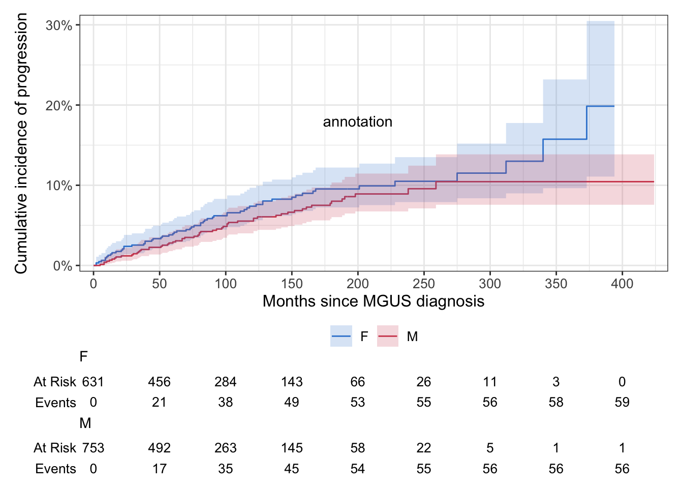
• Progression (pcm): Gray’s test p = 0.27. No convincing difference between men and women in the cumulative incidence of progression.
• Death: Gray’s test p < 0.001. Men have a higher cumulative incidence of death — the curves separate clearly.

So sex matters for the competing risk of death, not for progression itself — a distinction the naive analysis would have blurred.

Plot the CIF — ggcuminc() (the signature competing-risks figure)

Plot a cuminc() object directly with ggsurvfit::ggcuminc() — the publication-grade competing-risks curve, with confidence bands, a risk table, and Gray’s p placed on the panel:

library(survival)
library(tidycmprsk)
library(ggsurvfit)

mg <- mgus2
mg$etime <- ifelse(mg$pstat == 1, mg$ptime, mg$futime)
ecode <- with(mg, ifelse(pstat == 1, 1, ifelse(death == 1, 2, 0)))
mg$event <- factor(ecode, levels = c(0, 1, 2), labels = c("censor", "pcm", "death"))

ci_sex <- cuminc(Surv(etime, event) ~ sex, data = mg)

ggcuminc(ci_sex, outcome = "pcm") +
  add_confidence_interval() +
  add_risktable() +
  add_pvalue("annotation", location = "annotation", x = 200, y = 0.18) +
  scale_ggsurvfit() +
  scale_colour_manual(values = c("#3a86d4", "#d1495b")) +
  scale_fill_manual(values = c("#3a86d4", "#d1495b")) +
  labs(x = "Months since MGUS diagnosis", y = "Cumulative incidence of progression")

outcome = "pcm" picks the event to draw (you’d swap in "death" to plot the competing risk). The two curves sit close together — the visual companion to Gray’s p = 0.27.

Two hazards, two questions: cause-specific vs Fine-Gray

For covariate-adjusted modelling you have two regression models, and they answer different questions. Getting this right is the heart of competing risks.

ImportantWhich model? Etiology vs prediction

• Cause-specific hazard — fit a Cox model on the event of interest, treating competing events as censoring. It answers: “Among patients still alive and event-free, does this covariate change the rate at which the event occurs?” Use it for etiology / mechanism — is this factor biologically driving the event?
• Subdistribution hazard (Fine-Gray) — fit crr(), which keeps patients who had a competing event in the risk set. It answers: “Does this covariate change the cumulative incidence of the event?” Use it for prediction / risk — what is a patient’s actual probability of the event, given that they might die first?

They can point in different directions, and that is informative. A common report shows both.

Cause-specific Cox model

Fit a Cox model on progression, censoring death — this is the cause-specific hazard:

library(survival)

mg <- mgus2
mg$etime <- ifelse(mg$pstat == 1, mg$ptime, mg$futime)
ecode <- with(mg, ifelse(pstat == 1, 1, ifelse(death == 1, 2, 0)))
mg$event <- factor(ecode, levels = c(0, 1, 2), labels = c("censor", "pcm", "death"))

# Cause-specific: 1 = progression event, everything else (death + censor) = censored
mg$pcm_cs <- as.numeric(mg$event == "pcm")
cs_cox <- coxph(Surv(etime, pcm_cs) ~ sex + age, data = mg)
summary(cs_cox)$conf.int

     exp(coef) exp(-coef) lower .95 upper .95
sexM 0.9751755  1.0254564 0.6740140  1.410902
age  1.0131239  0.9870461 0.9968568  1.029657

age: cause-specific HR ≈ 1.01 per year (p = 0.11) — among patients still alive and event-free, age does not significantly change the rate of progression.

Fine-Gray subdistribution model

Now the Fine-Gray model with crr() — same covariates, but it models the cumulative incidence directly, keeping the patients who died in the risk set:

library(survival)
library(tidycmprsk)

mg <- mgus2
mg$etime <- ifelse(mg$pstat == 1, mg$ptime, mg$futime)
ecode <- with(mg, ifelse(pstat == 1, 1, ifelse(death == 1, 2, 0)))
mg$event <- factor(ecode, levels = c(0, 1, 2), labels = c("censor", "pcm", "death"))

fg <- crr(Surv(etime, event) ~ sex + age, data = mg, failcode = "pcm")
fg

Variable   Coef     SE      HR     95% CI       p-value    
sexM       -0.260   0.186   0.77   0.54, 1.11   0.16       
age        -0.017   0.006   0.98   0.97, 0.99   0.003      

failcode = "pcm" names the event of interest; the other levels are handled as the competing event / censoring automatically. Read the subdistribution hazard ratios (subHR):

• sex (male): subHR = 0.77, 95% CI 0.54–1.11, p = 0.16. No convincing sex effect on the cumulative incidence of progression — consistent with Gray’s test.
• age: subHR = 0.98 per year, 95% CI 0.97–0.99, p = 0.003. Each extra year of age is associated with a lower cumulative incidence of progression — a significant effect.

Why the two models disagree on age — and what it means

Look at what just happened with age:

Model	Effect of age	p	Interpretation
Cause-specific Cox	HR ≈ 1.01 (no effect)	0.11	Age doesn’t change the rate of progression
Fine-Gray subdistribution	subHR ≈ 0.98 (below 1)	0.003	Older patients have a lower cumulative incidence of progression

This is not a contradiction — it is the whole point of competing risks. Older patients progress at about the same rate while they are alive (cause-specific), but they are far more likely to die first (the competing risk), so fewer of them ever reach progression: their cumulative incidence is lower (Fine-Gray). The competing risk of death, captured by Fine-Gray and invisible to the cause-specific model, is doing the work.

Rule of thumb: report the cause-specific model when you ask “is this factor driving the biology of the event?”, and the Fine-Gray model when you ask “what is a patient’s actual risk of the event over time?” For a clinical risk discussion with a patient, Fine-Gray is usually the one you want.

Report

In 1384 patients with MGUS (mgus2), 115 progressed to a plasma-cell malignancy and 860 died first. Accounting for the competing risk of death, the cumulative incidence of progression was 6.4% (95% CI 5.1–7.8%) at 10 years and 10.0% at 20 years — substantially below the naive 1 − Kaplan-Meier estimate of 21% at 20 years, which incorrectly treats deaths as censored. Gray’s test showed no difference in the cumulative incidence of progression by sex (p = 0.27), but a higher incidence of death in men (p < 0.001). In a Fine-Gray subdistribution model, older age was associated with a lower cumulative incidence of progression (subHR = 0.98 per year, 95% CI 0.97–0.99, p = 0.003), driven by the higher competing mortality at older ages; the cause-specific hazard of progression did not change with age (HR = 1.01, p = 0.11).

NoteThe math behind the cumulative incidence function (optional)

For event type \(k\), the cause-specific hazard \(h_k(t)\) is the instantaneous rate of event \(k\) among those still event-free and alive. The cumulative incidence function for event \(k\) is built from its hazard weighted by the overall survival \(S(t)\) — the probability of still being at risk at all:

\[ F_k(t) = \int_0^t S(u^-)\, h_k(u)\, du \]

The key term is \(S(u^-)\), the probability of having had no event of any kind just before \(u\). It pulls the CIF below \(1 - \exp\!\big(-\int h_k\big)\) — the quantity \(1 - \mathrm{KM}\) estimates — because \(S\) shrinks as competing events occur, not just events of type \(k\). With no competing risks, \(S\) depends only on \(h_k\) and the two coincide; with competing risks, \(S\) falls faster and the CIF stays lower. The Fine-Gray subdistribution hazard \(\bar h_k(t)\) is instead defined to make \(F_k(t) = 1 - \exp\!\big(-\int \bar h_k\big)\), which is why a Fine-Gray model maps directly onto the cumulative incidence.

Which method when?

TipCompeting risks decision guide

• One event type, or competing events are rare (<10% of patients) → standard Kaplan-Meier and Cox are fine.
• A competing event can occur first and is common → use the cumulative incidence function (cuminc + ggcuminc), never 1 − KM, and compare groups with Gray’s test.
• Adjust for covariates, asking about the event rate / mechanism → cause-specific Cox (censor the competitor).
• Adjust for covariates, asking about the cumulative risk / for prediction → Fine-Gray crr() (subdistribution hazard).
• Recurrent events, or a composite “time to first of any event” → these are not competing risks; use standard or multi-state methods.

Try it live

Estimate the cumulative incidence function on mgus2 yourself — change the grouping variable, or plot outcome = "death" instead. The sandbox boots on first Run.

🟢 With an AI agent

Ask Prova “I have a survival dataset where patients can progress or die first — do a competing risks analysis: cumulative incidence function, Gray’s test, and a Fine-Gray model” — it answers with survival + tidycmprsk code you can run on your own data, with the event factor coded correctly. The runtime is the judge. Ask Prova →

Common issues

You treated the competing event as censoring (the classic mistake). Running survfit(Surv(time, progressed) ~ 1) and reading 1 − KM as the incidence of progression treats every death as “could still progress”. With substantial competing mortality this overstates the incidence — 21% vs 10% on mgus2. Build the multi-level event factor and use cuminc() instead.

You read 1 − KM as the cumulative incidence. Even after fitting the right model, don’t slip back into KM thinking: the survival curve’s complement is not the cumulative incidence when competing risks are present. The CIF from cuminc() is the only correct estimate of “fraction who had this event by time t”.

You confused the cause-specific and Fine-Gray hazard ratios. They answer different questions and can disagree (see age above). A cause-specific HR is about the rate of the event among those still at risk (etiology); a subdistribution HR is about the cumulative incidence (prediction). State which one you fitted, and don’t interpret a Fine-Gray subHR as if it were a cause-specific rate ratio.

cuminc() errors on the event variable. tidycmprsk needs the event to be a factor whose first level is the censoring code (here "censor"). A numeric event, or a factor with the wrong level order, fails or returns nonsense — set levels = c("censor", ...) explicitly.

Frequently asked questions

NoteWhat is the difference between a competing risk and censoring?

A censored patient is one you stopped observing (study ended, lost to follow-up) who could still have the event of interest if followed longer — standard survival analysis handles this. A competing risk is a different event (usually death) that makes the event of interest impossible: a patient who dies before progressing can never progress. Treating a competing event as censoring assumes the impossible and overestimates the incidence of the event of interest.

NoteWhy does 1 minus Kaplan-Meier overestimate risk with competing events?

Because the Kaplan-Meier estimator assumes everyone removed from the risk set was merely censored and could still have the event. When competing events (deaths) are censored this way, KM credits those patients with a future chance of the event they can never have, so 1 − KM climbs too high. The cumulative incidence function only counts events that actually occur among patients still alive and at risk, giving the correct, lower estimate — on mgus2, 10% vs the naive 21% at 20 years.

NoteCause-specific vs Fine-Gray — which model should I use?

Use the cause-specific Cox model (censor the competing event) when you want etiology — does this covariate change the rate at which the event occurs among those still at risk? Use the Fine-Gray subdistribution model (crr()) when you want prediction / cumulative risk — does this covariate change a patient’s actual probability of the event over time, given they might die first? They answer different questions and can disagree; many analyses report both, with Fine-Gray preferred for clinical risk communication.

NoteWhat R package should I use for competing risks?

tidycmprsk is the modern choice: cuminc() for the cumulative incidence function and Gray’s test, crr() for the Fine-Gray subdistribution model, with tidy output. Pair it with ggsurvfit for publication-grade ggcuminc() plots (confidence bands, risk tables, on-plot p-values). The base survival package supplies the data and the Surv() / coxph() engine for the cause-specific model.

NoteHow do I code the event variable for tidycmprsk?

Make it a factor whose first level is the censoring code. Build one event-time variable (the progression time if progressed, else the follow-up time) and one event code (e.g. 0 = censored, 1 = event of interest, 2 = competing event), then factor(code, levels = c(0,1,2), labels = c("censor","pcm","death")). The “censor first” ordering is mandatory — cuminc() and crr() rely on it.

Test your understanding

ImportantPractice

1. Run it. In the live cell below, estimate the cumulative incidence by sex and read off the progression CIF at 120 months for each sex. Fill the blank with the event of interest.
2. Interpret. A naive 1 − KM analysis reports a 5-year incidence of progression of 18%, but the cumulative incidence function reports 11%. Explain in one sentence why they differ and which is correct.

NoteHint

The event of interest is progression, coded "pcm" in the factor. tidy(ci, times = 120) returns one row per stratum × outcome; filter to outcome == "pcm" to read the progression CIF for each sex.

NoteSolution

ci <- cuminc(Surv(etime, event) ~ sex, data = mg)
tidy(ci, times = 120)[tidy(ci, times = 120)$outcome == "pcm", ]
#> Female CIF ~ 0.074, Male CIF ~ 0.055 at 120 months — close together,
#> matching Gray's test p = 0.27 (no convincing sex difference in progression).

For question 2: the 1 − KM estimate (18%) overstates the incidence because it treats patients who died before progressing as if they could still progress; the cumulative incidence function (11%) is correct because it accounts for the competing risk of death removing those patients from risk.

TipQuick check

A Fine-Gray model gives a subdistribution hazard ratio of 0.80 (95% CI 0.68–0.94) for a treatment. What does this mean clinically?

NoteShow answer

The treatment is associated with a 20% lower cumulative incidence of the event of interest over time ((1 − 0.80) × 100), accounting for the competing risk. Because the 95% CI (0.68–0.94) lies entirely below 1, the reduction is statistically convincing. Note this is a statement about cumulative risk, not about the event rate among those still at risk — that would be the cause-specific hazard.

Conclusion

Competing risks turn up whenever a patient can fail from more than one cause and one event blocks another — most often death before the event of interest. The fix is disciplined: build a single event factor (censor level first), summarise risk with the cumulative incidence function (cuminc + ggcuminc), never 1 − Kaplan-Meier, and compare groups with Gray’s test. For covariate adjustment, choose by the question: the cause-specific Cox model for the event rate (etiology), the Fine-Gray model for the cumulative incidence (prediction) — and remember they can disagree, as age did on mgus2. Get the event coding right and the rest follows.

Related lessons

• Kaplan-Meier estimation — the survival curve competing risks corrects; understand it first. · Cox proportional hazards — the engine behind the cause-specific model. · What is survival analysis? — censoring, hazard, and survival functions explained. · Restricted mean survival time — another way to summarise survival when the proportional-hazards story is awkward. · CDISC ADTTE for regulatory submissions — structuring competing-events data for a clinical submission.
• Go further: Survival Analysis — the full series. · Biostatistics — the pillar.

Was this page helpful?

Prove you can do it. Master the whole Survival Analysis in R series — track your path, build projects, and earn a certificate.

Start free →

Go Pro — unlimited Prova on your own data and a verifiable certificate that proves the skill.

from $15/mo billed yearly

Go Pro →

✓ You're Pro — keep going. The runtime is the judge.

Ready to level up?

Try this on your own data with Prova — the runtime is the judge.Open Prova →

Get new R & Python lessons by email

Practical, reproducible, no spam. Unsubscribe anytime.

Double opt-in. We never share your email.

Share this pageXLinkedInRedditHN

Note

Every result on this page was produced by the code shown, run at build time against a pinned R environment — copy any block, or hit Try ▸ / Run, to reproduce it yourself.