Complete Survival Analysis Example in R: Kaplan-Meier, Log-Rank, Cox — Start to Finish

One end-to-end project on the lung-cancer data — frame the question, prepare the data, estimate Kaplan-Meier curves and medians, run the log-rank test, fit and interpret a Cox model, check proportional hazards, and write the publication-ready report

A complete, worked survival analysis in R from start to finish on the NCCTG lung-cancer dataset. Frame the question and build the Surv() response, estimate Kaplan-Meier survival curves and median survival by sex, compare groups with the log-rank test, fit univariate and multivariable Cox proportional hazards models and interpret the hazard ratios, validate the proportional-hazards assumption with cox.zph and ggcoxzph, and assemble the publication-ready figure and report paragraph — every step cross-linked to the lesson that teaches it.

TipKey takeaways

• This capstone runs a complete survival analysis end to end on the NCCTG lung-cancer data — the exact sequence you would follow on your own time-to-event study, with each step linked to the lesson that teaches it in depth.
• The workflow: frame the question → prepare the data (Surv) → Kaplan-Meier curves + median survival → log-rank test → Cox model (hazard ratios) → check proportional hazards → report.
• The result on lung: median survival 270 days (men) vs 426 days (women); the log-rank test confirms the gap (χ²(1) = 10.3, p = 0.001); a multivariable Cox model gives female sex HR ≈ 0.58 (a 42% lower hazard) and ECOG score HR ≈ 1.59 (a 59% higher hazard per point), with age dropping out after adjustment.
• The proportional-hazards assumption holds for the final model (cox.zph GLOBAL p = 0.22), so the hazard ratios are trustworthy.
• Two packages do everything: survival (the models and tests) and survminer (the publication-ready ggsurvplot, ggforest, and ggcoxzph figures).

Introduction

You have learned the pieces — Kaplan-Meier curves, the log-rank test, the Cox model, the PH diagnostics. This lesson is the project that puts them together: a single, complete survival analysis from raw data to a paragraph you could paste into a paper.

We will answer one clinical question on the NCCTG lung-cancer data — which patient factors change the risk of death, and how much longer do women survive than men? — by walking the full workflow:

1. Frame the question and prepare the data — build the Surv(time, status) response.
2. Estimate survival with Kaplan-Meier curves; read median survival and its 95% CI.
3. Compare the sexes with the log-rank test.
4. Model the effect of several covariates at once with Cox regression — hazard ratios with CIs.
5. Validate the model: test the proportional-hazards assumption.
6. Report — the publication figure and the write-up paragraph.

Each step is tight on purpose: the teaching depth lives in the linked lessons. Here you see them working together on one dataset to a finished result. Two packages carry the whole analysis — survival (models and tests) and survminer (the figures).

Step 1 — Frame the question and prepare the data

The question. In 228 patients with advanced lung cancer, does survival differ by sex, and which clinical factors (age, performance status, weight loss) raise or lower the hazard of death? The outcome is time to death, with censoring for patients still alive at last follow-up — exactly the setting survival analysis is built for.

The data. We use lung, the dataset that ships with the survival package. It attaches automatically, so you reference lung directly — no data() call needed (see preparing survival data for the full data-prep checklist):

library(survival)

head(lung)

  inst time status age sex ph.ecog ph.karno pat.karno meal.cal wt.loss
1    3  306      2  74   1       1       90       100     1175      NA
2    3  455      2  68   1       0       90        90     1225      15
3    3 1010      1  56   1       0       90        90       NA      15
4    5  210      2  57   1       1       90        60     1150      11
5    1  883      2  60   1       0      100        90       NA       0
6   12 1022      1  74   1       1       50        80      513       0

The columns this analysis uses:

• time — follow-up time in days.
• status — censoring status: 1 = censored (alive at last follow-up), 2 = dead (the event).
• sex — 1 = male, 2 = female.
• age — age in years.
• ph.ecog — ECOG performance score (0 = fully active … higher = more impaired).
• ph.karno — Karnofsky performance score (higher = better function).
• wt.loss — weight loss in the last six months (kg).

A quick sanity check — how many events, and how much missingness in the covariates we will model:

library(survival)

# Events vs censored (status: 1 = censored, 2 = dead)
table(status = lung$status)

status
  1   2 
 63 165 

# Missing values per covariate we'll use
colSums(is.na(lung[c("age", "sex", "ph.ecog", "ph.karno", "wt.loss")]))

     age      sex  ph.ecog ph.karno  wt.loss 
       0        0        1        1       14 

There are 165 deaths among 228 patients (the rest censored), and a handful of missing covariate values — worth noting now, because a Cox model uses complete cases and will quietly drop those rows.

Build the Surv() response

Every survival model takes a time–event pair on the left-hand side, built with Surv(time, status). A + after a time marks a censored patient (alive when last seen):

library(survival)

head(Surv(lung$time, lung$status))

[1]  306   455  1010+  210   883  1022+

306 and 455 are deaths; 1010+ is censored — that patient was alive at 1010 days, so we know only that their survival exceeds 1010 days. This object is the response for everything that follows.

Step 2 — Estimate survival: Kaplan-Meier

Estimate the survival curves with survfit(), overall and by sex. The printout gives the headline summary — the median survival and its 95% CI per group (the depth is in Kaplan-Meier estimation and median survival & CI):

library(survival)

# Overall, then by sex
survfit(Surv(time, status) ~ 1, data = lung)

Call: survfit(formula = Surv(time, status) ~ 1, data = lung)

       n events median 0.95LCL 0.95UCL
[1,] 228    165    310     285     363

fit <- survfit(Surv(time, status) ~ sex, data = lung)
fit

Call: survfit(formula = Surv(time, status) ~ sex, data = lung)

        n events median 0.95LCL 0.95UCL
sex=1 138    112    270     212     310
sex=2  90     53    426     348     550

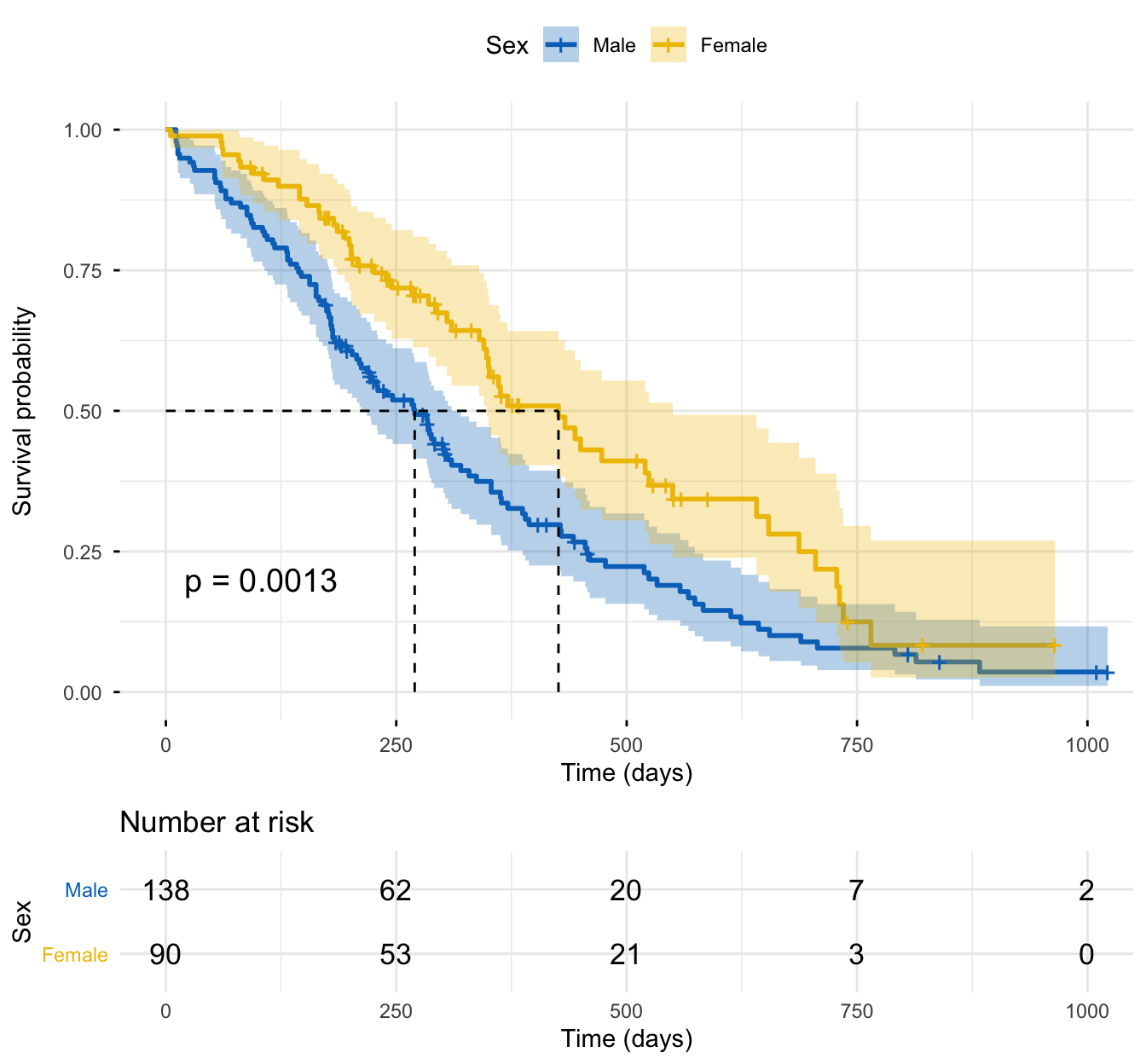
Read it: overall median survival is 310 days. Split by sex, median survival is 270 days for men (sex = 1) and 426 days for women (sex = 2) — women survive markedly longer. The 95% CIs (212–310 for men, 348–550 for women) barely overlap, hinting at a real difference we will test in Step 3.

The publication figure: ggsurvplot()

Numbers are precise, but survival is read from the curve. survminer’s ggsurvplot() draws the Kaplan-Meier curves with everything a reviewer expects — confidence bands, the risk table, the median lines, and the log-rank p-value — on one panel (the full styling guide is in publication-ready survival curves):

library(survival)
library(survminer)

fit <- survfit(Surv(time, status) ~ sex, data = lung)

ggsurvplot(
  fit,
  data = lung,
  risk.table = TRUE,        # number at risk under the plot
  conf.int = TRUE,          # 95% confidence bands
  pval = TRUE,              # log-rank p-value, on the plot
  surv.median.line = "hv",  # dashed median-survival guides
  palette = "jco",          # colourblind-safe journal palette
  legend.labs = c("Male", "Female"),
  legend.title = "Sex",
  xlab = "Time (days)",
  ylab = "Survival probability",
  ggtheme = theme_minimal()
)

The female curve sits above the male curve at every time point; the dashed median lines meet the x-axis at 270 and 426 days; the log-rank p = 0.0013 on the panel already previews Step 3. The risk table shows how few patients remain late in follow-up — which is why the bands fan out at the tail.

Step 3 — Compare the groups: the log-rank test

The plot suggests women survive longer; the log-rank test decides whether the gap is real. Run it with survdiff(), same formula as survfit() (full lesson: log-rank test):

library(survival)

survdiff(Surv(time, status) ~ sex, data = lung)

Call:
survdiff(formula = Surv(time, status) ~ sex, data = lung)

        N Observed Expected (O-E)^2/E (O-E)^2/V
sex=1 138      112     91.6      4.55      10.3
sex=2  90       53     73.4      5.68      10.3

 Chisq= 10.3  on 1 degrees of freedom, p= 0.001 

Read it: men had 112 observed vs 91.6 expected deaths (more than expected), women 53 vs 73.4 (fewer) — that mismatch is the signal. It accumulates into χ² = 10.3 on 1 df, p = 0.001. Because p < 0.05 we reject the null of equal survival: women survive significantly longer than men. The log-rank test gives the p-value but no effect size — for how much the risk differs, and to adjust for other factors, we move to the Cox model.

Step 4 — Model the covariates: Cox proportional hazards

The Cox model handles continuous and categorical predictors and adjusts each effect for the others, returning a hazard ratio (HR) per factor (full lesson: Cox proportional hazards). Recall: HR < 1 = lower hazard (better survival), HR > 1 = higher hazard (worse), HR = 1 or a CI crossing 1 = no convincing effect.

Scan the covariates one at a time (univariate)

Start by fitting a univariate Cox model for each candidate covariate and tabulating the HRs — a quick screen for which factors matter:

library(survival)

covariates <- c("age", "sex", "ph.ecog", "ph.karno", "wt.loss")
univ_formulas <- sapply(covariates,
                        function(x) as.formula(paste("Surv(time, status) ~", x)))
univ_models <- lapply(univ_formulas, function(f) coxph(f, data = lung))

univ_results <- lapply(univ_models, function(m) {
  s <- summary(m)
  HR    <- signif(s$coef[2], 2)
  lower <- signif(s$conf.int[, "lower .95"], 2)
  upper <- signif(s$conf.int[, "upper .95"], 2)
  p     <- signif(s$wald["pvalue"], 2)
  c(HR = paste0(HR, " (", lower, "-", upper, ")"), p.value = p)
})
as.data.frame(t(as.data.frame(univ_results, check.names = FALSE)))

                       HR p.value.pvalue
age               1 (1-1)          0.042
sex      0.59 (0.42-0.82)         0.0015
ph.ecog       1.6 (1.3-2)        2.7e-05
ph.karno    0.98 (0.97-1)          0.005
wt.loss        1 (0.99-1)           0.83

What this tells us: sex, ph.ecog, ph.karno, and (just) age carry significant univariate effects; wt.loss does not (p = 0.83). ph.ecog (HR ≈ 1.6) and age (HR ≈ 1.02) raise the hazard; sex (HR ≈ 0.59) and ph.karno (HR ≈ 0.98) lower it. But univariate effects can be confounded — ph.ecog and ph.karno are two views of the same performance status — so the real test is fitting them together.

Fit them together (multivariable)

Fit the clinically relevant covariates at once, so each effect is adjusted for the rest:

library(survival)

res.full <- coxph(Surv(time, status) ~ age + sex + ph.ecog + ph.karno + wt.loss, data = lung)
summary(res.full)

Call:
coxph(formula = Surv(time, status) ~ age + sex + ph.ecog + ph.karno + 
    wt.loss, data = lung)

  n= 213, number of events= 151 
   (15 observations effacées parce que manquantes)

              coef exp(coef)  se(coef)      z Pr(>|z|)    
age       0.015157  1.015273  0.009763  1.553 0.120538    
sex      -0.631422  0.531835  0.177134 -3.565 0.000364 ***
ph.ecog   0.740204  2.096364  0.191332  3.869 0.000109 ***
ph.karno  0.015251  1.015368  0.009797  1.557 0.119553    
wt.loss  -0.009298  0.990745  0.006699 -1.388 0.165168    
---
Signif. codes:  0 '***' 0.001 '**' 0.01 '*' 0.05 '.' 0.1 ' ' 1

         exp(coef) exp(-coef) lower .95 upper .95
age         1.0153     0.9850    0.9960    1.0349
sex         0.5318     1.8803    0.3758    0.7526
ph.ecog     2.0964     0.4770    1.4408    3.0502
ph.karno    1.0154     0.9849    0.9961    1.0351
wt.loss     0.9907     1.0093    0.9778    1.0038

Concordance= 0.64  (se = 0.026 )
Likelihood ratio test= 33.53  on 5 df,   p=3e-06
Wald test            = 32.27  on 5 df,   p=5e-06
Score (logrank) test = 32.83  on 5 df,   p=4e-06

Interpret the adjusted output: only sex (HR = 0.53, p = 0.0004) and ph.ecog (HR = 2.10, p = 0.0001) survive adjustment. age, ph.karno, and wt.loss all become non-significant (their CIs cross 1) — once you know a patient’s sex and ECOG score, they add little. Note also n = 213, not 228: coxph() dropped 15 patients with a missing covariate (complete-case analysis). A leaner model is both simpler and avoids losing rows to wt.loss’s missingness — the formal way to choose it is Cox model building & selection. Here we keep the two strong, clinically interpretable factors plus age, and carry age + sex + ph.ecog forward as the final model.

library(survival)

res.cox <- coxph(Surv(time, status) ~ age + sex + ph.ecog, data = lung)
summary(res.cox)

Call:
coxph(formula = Surv(time, status) ~ age + sex + ph.ecog, data = lung)

  n= 227, number of events= 164 
   (1 observation effacée parce que manquante)

             coef exp(coef)  se(coef)      z Pr(>|z|)    
age      0.011067  1.011128  0.009267  1.194 0.232416    
sex     -0.552612  0.575445  0.167739 -3.294 0.000986 ***
ph.ecog  0.463728  1.589991  0.113577  4.083 4.45e-05 ***
---
Signif. codes:  0 '***' 0.001 '**' 0.01 '*' 0.05 '.' 0.1 ' ' 1

        exp(coef) exp(-coef) lower .95 upper .95
age        1.0111     0.9890    0.9929    1.0297
sex        0.5754     1.7378    0.4142    0.7994
ph.ecog    1.5900     0.6289    1.2727    1.9864

Concordance= 0.637  (se = 0.025 )
Likelihood ratio test= 30.5  on 3 df,   p=1e-06
Wald test            = 29.93  on 3 df,   p=1e-06
Score (logrank) test = 30.5  on 3 df,   p=1e-06

The final model in plain language:

• sex: HR = 0.58, 95% CI 0.41–0.80, p = 0.001. Holding age and ECOG score constant, being female cuts the hazard of death by ~42% — the strongest, most robust signal.
• ph.ecog: HR = 1.59, 95% CI 1.27–1.99, p < 0.001. Each one-point worsening of the performance score raises the hazard by ~59% — a strong bad prognostic factor.
• age: HR = 1.01, 95% CI 0.99–1.03, p = 0.23. After adjustment, age is not significant (the CI includes 1); its univariate effect was explained by the other covariates.

The forest plot: ggforest()

The signature Cox figure shows every covariate’s HR, CI, and p-value on one panel, with the reference line at HR = 1 — left of it is protective, right of it is harmful:

library(survival)
library(survminer)

res.cox <- coxph(Surv(time, status) ~ age + sex + ph.ecog, data = lung)
ggforest(res.cox, data = lung)

At a glance: sex well left of the line (protective), ph.ecog right of it (harmful), age straddling it (no clear effect) — exactly what the numbers said.

Step 5 — Validate the model: proportional hazards

Every hazard ratio above assumes the effect is constant over time — the proportional-hazards (PH) assumption. Before trusting the HRs, test it with cox.zph() (scaled Schoenfeld residuals), which gives a per-covariate test and a GLOBAL test (full lesson: testing PH assumptions):

library(survival)

res.cox <- coxph(Surv(time, status) ~ age + sex + ph.ecog, data = lung)
test.ph <- cox.zph(res.cox)
test.ph

        chisq df    p
age     0.188  1 0.66
sex     2.305  1 0.13
ph.ecog 2.054  1 0.15
GLOBAL  4.464  3 0.22

Read it: the decision rule is p ≥ 0.05 → PH holds, p < 0.05 → PH violated. Every per-covariate test is non-significant (age p = 0.66, sex p = 0.13, ECOG p = 0.15) and the GLOBAL test is p = 0.22 (χ² = 4.46 on 3 df). The assumption is supported — the hazard ratios can be read as constant over time.

NoteWhy the leaner model also validates cleaner

The full five-covariate model in Step 4 was almost fine, but cox.zph() flagged ph.karno with p = 0.03 — a mild PH violation. Dropping the redundant, non-significant covariates didn’t just simplify the model; it removed the one variable whose effect drifted over time. A parsimonious model is often a better-behaved one.

See it on the ggcoxzph() plot — a flat smoothing line in each panel means no time trend:

library(survival)
library(survminer)

res.cox <- coxph(Surv(time, status) ~ age + sex + ph.ecog, data = lung)
test.ph <- cox.zph(res.cox)

ggcoxzph(test.ph)

All three splines are essentially flat and stay inside the band — no systematic trend with time, matching the non-significant cox.zph() p-values. As a final check, influential observations (ggcoxdiagnostics(), dfbeta) show no single patient distorting the fit:

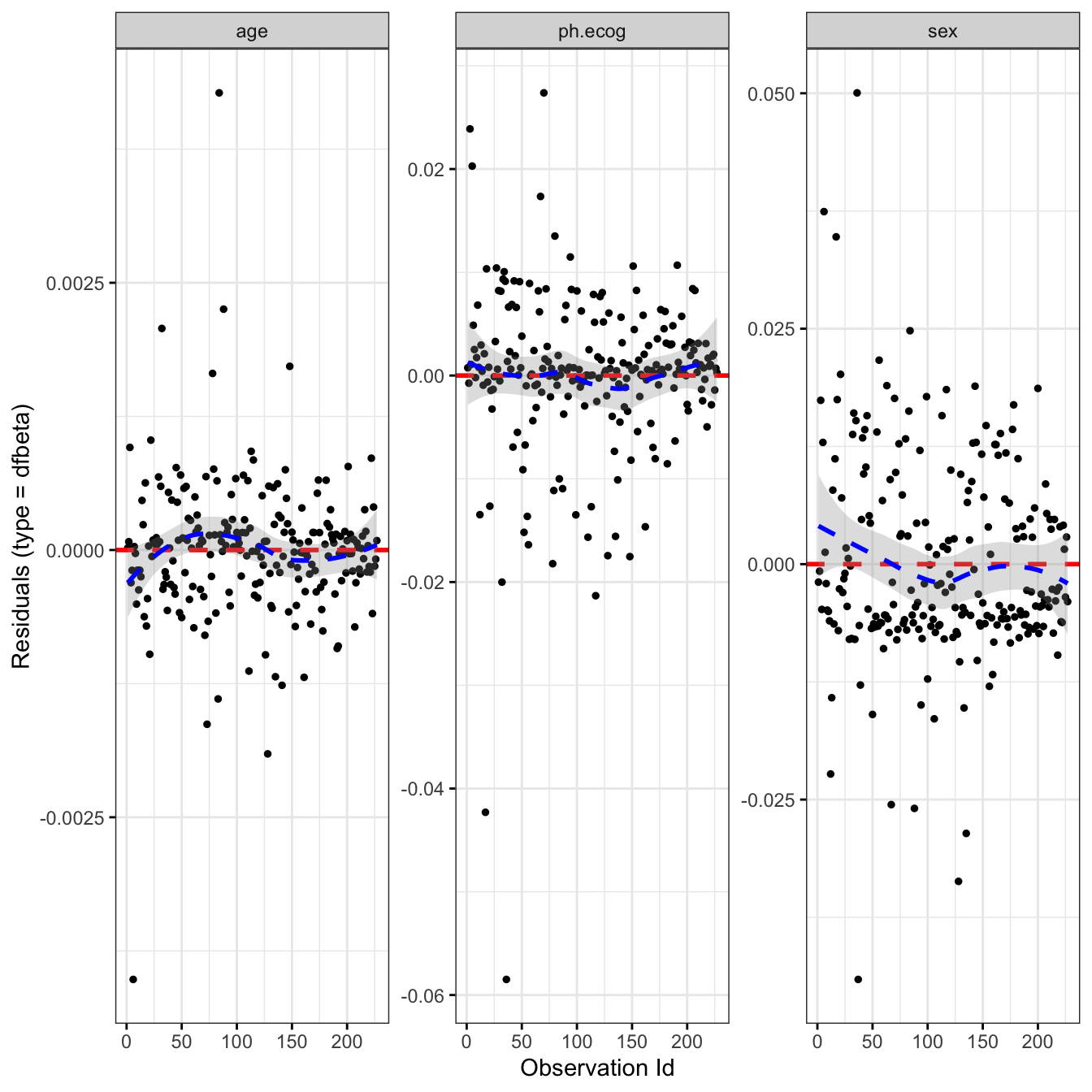
library(survival)
library(survminer)

res.cox <- coxph(Surv(time, status) ~ age + sex + ph.ecog, data = lung)

ggcoxdiagnostics(res.cox, type = "dfbeta", linear.predictions = FALSE)

A handful of points for age and ph.ecog are larger than the rest, but none is large relative to its coefficient — no patient needs removing. The model is validated.

Step 6 — Report

The whole analysis, written up the way it would appear in a clinical paper:

Overall survival in 228 patients with advanced lung cancer (NCCTG data; 165 deaths) was estimated by the Kaplan-Meier method. Median survival was 270 days (95% CI 212–310) for men and 426 days (95% CI 348–550) for women, a difference that was statistically significant by the log-rank test (χ²(1) = 10.3, p = 0.001). A multivariable Cox proportional hazards model (n = 227, 164 events) adjusting for age, sex, and ECOG performance score showed that female sex was associated with a significantly lower hazard of death (HR = 0.58, 95% CI 0.41–0.80, p = 0.001) and a higher ECOG score with a higher hazard (HR = 1.59, 95% CI 1.27–1.99, p < 0.001); age was not significant after adjustment (HR = 1.01, 95% CI 0.99–1.03, p = 0.23). The proportional-hazards assumption was satisfied (scaled Schoenfeld residuals, GLOBAL χ²(3) = 4.46, p = 0.22), and influence diagnostics revealed no unduly influential observations.

That paragraph — medians with CIs, the log-rank result, the adjusted hazard ratios, and the assumption check — is a complete, defensible survival analysis.

What you would do next

The lung analysis is clean because death is the only event and PH holds. Real studies often add a wrinkle — and each has a lesson in this series:

• Patients can die of other causes, not the event of interest → competing risks (cumulative incidence, the Fine-Gray model) instead of plain Kaplan-Meier.
• The hazard ratio is not constant (curves cross, a delayed effect) → compare restricted mean survival time (RMST), or use a time-varying covariate / stratified Cox model.
• You want a smooth survival function or to extrapolate beyond follow-up → parametric survival models.
• You are designing the study, not analysing it → designing a survival study and choosing a survival endpoint.

Try it live

Run the whole analysis yourself — change the grouping variable, add a covariate to the Cox model, or swap the final model. The sandbox boots on first Run.

🟢 With an AI agent

Ask Prova “run a complete survival analysis on my data — Kaplan-Meier curves with median survival, a log-rank test, a Cox model with hazard ratios, and a proportional-hazards check — and write me the report paragraph” — it answers with survival + survminer code you can run on your own data. The runtime is the judge. Ask Prova →

Common issues

Your Cox model “lost” patients — the n shrank. coxph() uses complete cases: any patient with a missing value in any covariate is dropped. The full five-covariate model fell to n = 213 (15 dropped), mostly because wt.loss is missing for some patients; the leaner age + sex + ph.ecog model kept n = 227. Always check model$n against nrow(lung), and prefer a model with fewer, more-complete covariates (or impute) rather than silently analysing a different sample.

You read the hazard ratio direction backwards. In lung, sex is 1 = male, 2 = female, so the HR is female vs male. HR = 0.58 means females have a lower hazard (better survival) — protective. With a factor, R uses the first level as the reference; check the coding before you call a factor “harmful”.

You reported the hazard ratios without checking proportional hazards. A Cox HR is only meaningful if the effect is constant over time. Always run cox.zph() (and look at ggcoxzph()): a significant test or a sloped residual plot means the single HR is a misleading time-average — fix it with stratification or a time-varying term (see testing PH assumptions), don’t just publish the number.

Frequently asked questions

NoteHow do I do a complete survival analysis in R?

Follow this sequence: (1) build the response with Surv(time, status); (2) estimate Kaplan-Meier curves with survfit(Surv(time, status) ~ group, data) and read the median survival; (3) compare groups with the log-rank test, survdiff(); (4) fit a Cox model, coxph(), and interpret the hazard ratios with 95% CIs; (5) check the proportional-hazards assumption with cox.zph() and ggcoxzph(); (6) report the medians, the log-rank result, the adjusted hazard ratios, and the PH check. Two packages cover it all: survival and survminer.

NoteKaplan-Meier or Cox — which should I do first?

Kaplan-Meier first. It describes survival in each group (the curves and median survival) with no assumptions, and the log-rank test tells you whether groups differ. Then fit the Cox model to quantify the effect as a hazard ratio, use continuous predictors, and adjust for several covariates at once. Kaplan-Meier is description; Cox is the modelling step that builds on it.

NoteWhat does the lung dataset contain for survival analysis?

lung (in the survival package) holds survival data on 228 advanced lung-cancer patients from the North Central Cancer Treatment Group: time (follow-up in days), status (1 = censored, 2 = dead), sex (1 = male, 2 = female), age, and performance-status covariates ph.ecog, ph.karno, pat.karno, meal.cal, and wt.loss. It attaches automatically with the package, so you reference lung directly.

NoteHow do I interpret the hazard ratios in this analysis?

A hazard ratio is a multiplicative effect on the risk of death. HR = 0.58 for female sex means women have a 42% lower hazard than men ((1 − 0.58) × 100) — protective. HR = 1.59 for ECOG score means each one-point worsening raises the hazard by 59% — harmful. HR = 1.01 for age with a CI that includes 1 means no convincing effect. Always read an HR together with its 95% confidence interval and p-value.

NoteWhich R packages do I need for a full survival analysis?

Two. survival does the modelling and testing: Surv(), survfit() (Kaplan-Meier), survdiff() (log-rank), coxph() (Cox), and cox.zph() (PH test). survminer does the publication-grade figures: ggsurvplot() (KM curves with risk table, CI, median lines, p-value), ggforest() (hazard-ratio forest plot), and ggcoxzph() / ggcoxdiagnostics() (model diagnostics). Both ship the lung dataset used here.

Test your understanding

ImportantPractice

1. Run it. In the live cell below, extend the analysis: fit the final Cox model adding wt.loss as a fourth covariate, then check proportional hazards. Fill the blank. Is wt.loss a significant predictor after adjustment, and does the GLOBAL cox.zph() test still support PH?
2. Interpret. Your Cox model reports, for a treatment indicator, HR = 0.65 (95% CI 0.48–0.88, p = 0.005), and cox.zph() gives a GLOBAL p = 0.40. In plain words, what is the treatment effect, is it statistically convincing, and can you trust the hazard ratio?

NoteHint

Fill the blank with wt.loss. In summary(), read wt.loss’s exp(coef) (the HR) and its p-value — a CI crossing 1 (or p ≥ 0.05) means no convincing effect. In cox.zph(), read the GLOBAL row: p ≥ 0.05 means PH is supported.

NoteSolution

res.cox <- coxph(Surv(time, status) ~ age + sex + ph.ecog + wt.loss, data = lung)
summary(res.cox)
#> wt.loss HR ~ 0.99, p ~ 0.5 — NOT significant after adjustment (CI crosses 1);
#> sex and ph.ecog remain the strong predictors. n drops to ~214 (wt.loss missingness).
cox.zph(res.cox)
#> GLOBAL p > 0.05 — the proportional-hazards assumption is still supported.

wt.loss adds nothing once sex and ECOG score are in the model, and it costs you rows to missingness — a good reason to leave it out. PH still holds overall.

For question 2: HR = 0.65 means a 35% lower hazard of death in the treated group ((1 − 0.65) × 100) — a protective treatment effect. It is statistically convincing: the 95% CI (0.48–0.88) lies entirely below 1 and p = 0.005. And because cox.zph() GLOBAL p = 0.40 (≥ 0.05), proportional hazards holds, so the single hazard ratio is trustworthy — you can report it as a constant effect over follow-up.

TipQuick check

You run a survival analysis and find the Kaplan-Meier curves separate clearly, but the log-rank test gives p = 0.18. A reviewer asks for the hazard ratio “to be sure”. What is the right next step?

NoteShow answer

Fit a Cox model to get the hazard ratio with its 95% CI — the log-rank test gives only a p-value, not an effect size. But interpret it honestly: a non-significant log-rank test (p = 0.18) means there isn’t strong evidence the curves differ, so expect the Cox HR’s confidence interval to cross 1. If the curves clearly cross, the log-rank test loses power and PH is likely violated — check cox.zph(), and consider a weighted log-rank test or RMST rather than forcing a single HR.

Conclusion

You have run a complete survival analysis in R from start to finish: framed the question, built the Surv(time, status) response, estimated Kaplan-Meier curves and read median survival (270 vs 426 days), confirmed the difference with the log-rank test (p = 0.001), fit and interpreted a multivariable Cox model (female sex HR 0.58, ECOG HR 1.59), validated it against the proportional-hazards assumption (GLOBAL p = 0.22), and assembled the publication-ready figure and report paragraph. That sequence — describe, compare, model, validate, report — is the backbone of every time-to-event study; swap in your own data and the same six steps carry you to a defensible result. When your data adds a wrinkle (competing events, crossing curves, a parametric form), the what you’d do next lessons take it from here.

Related lessons

• Kaplan-Meier estimation — estimate survival curves and read median survival, the descriptive heart of Step 2. · Log-rank test — the formal group comparison in Step 3 (the p-value on the plot). · Cox proportional hazards — fit and interpret hazard ratios, the modelling in Step 4. · Testing PH assumptions — the diagnostics that validate the model in Step 5. · Publication-ready survival curves — the full ggsurvplot styling toolkit for the figures.
• Go further: Survival Analysis — the full series. · Biostatistics — the pillar.

Was this page helpful?

Prove you can do it. Master the whole Survival Analysis in R series — track your path, build projects, and earn a certificate.

Start free →

Go Pro — unlimited Prova on your own data and a verifiable certificate that proves the skill.

from $15/mo billed yearly

Go Pro →

✓ You're Pro — keep going. The runtime is the judge.

Ready to level up?

Try this on your own data with Prova — the runtime is the judge.Open Prova →

Get new R & Python lessons by email

Practical, reproducible, no spam. Unsubscribe anytime.

Double opt-in. We never share your email.

Share this pageXLinkedInRedditHN

Note

Every result on this page was produced by the code shown, run at build time against a pinned R environment — edit any block and Run to reproduce it yourself.