Logistic Regression Assumptions and Diagnostics in R
After you fit a logistic model, check it: the binary outcome, the linearity of the logit, influential points (Cook’s distance), and multicollinearity (VIF) — each with the fix when it fails
Biostatistics
Check the assumptions of a logistic regression in R: a binary outcome, a linear relationship between each continuous predictor and the logit, no influential observations, and no multicollinearity. Inspect logit-linearity scatter plots, Cook’s distance and standardized residuals, and VIF — with the workaround for each violation. Run it all live.
Published
June 23, 2026
Modified
July 7, 2026
TipKey takeaways
A logistic regression makes four assumptions — check them before you trust the model.
Binary outcome: the response must have exactly two classes.
Linearity of the logit: each continuous predictor should be linearly related to the log-odds of the outcome — check with a predictor-vs-logit scatter plot + loess.
No influential points: screen with Cook’s distance and standardized residuals (|value| > 3 is a possible outlier).
No multicollinearity: predictors shouldn’t be strongly correlated with each other — check car::vif() (> 5 is problematic).
Each violation has a fix: transform/spline a non-linear predictor, investigate an influential point, remove a collinear predictor.
Introduction
Fitting a logistic regression gives you odds ratios and p-values — but those are only trustworthy if the model’s assumptions hold. Logistic regression has its own diagnostic checklist, related to but different from linear regression’s.
This lesson walks through the four assumptions, how to check each in R, and — the practical part — what to do when one fails.
The model to check
We reuse the diabetes model from the logistic regression lesson — glm() on the clinical predictors — and grab its predicted probabilities:
data("PimaIndiansDiabetes2", package ="mlbench")diabetes_data <-na.omit(PimaIndiansDiabetes2)model <-glm(diabetes ~ ., data = diabetes_data, family = binomial)probabilities <-predict(model, type ="response")head(probabilities)
Binary outcome — the response has exactly two classes (here pos/neg). ✔ by design.
Linearity of the logit — each continuous predictor is linearly related to the log-odds of the outcome.
No influential values — no extreme points distorting the fit.
No multicollinearity — predictors aren’t strongly correlated with each other.
Assumption 1 is automatic; the next three need checking.
Linearity of the logit
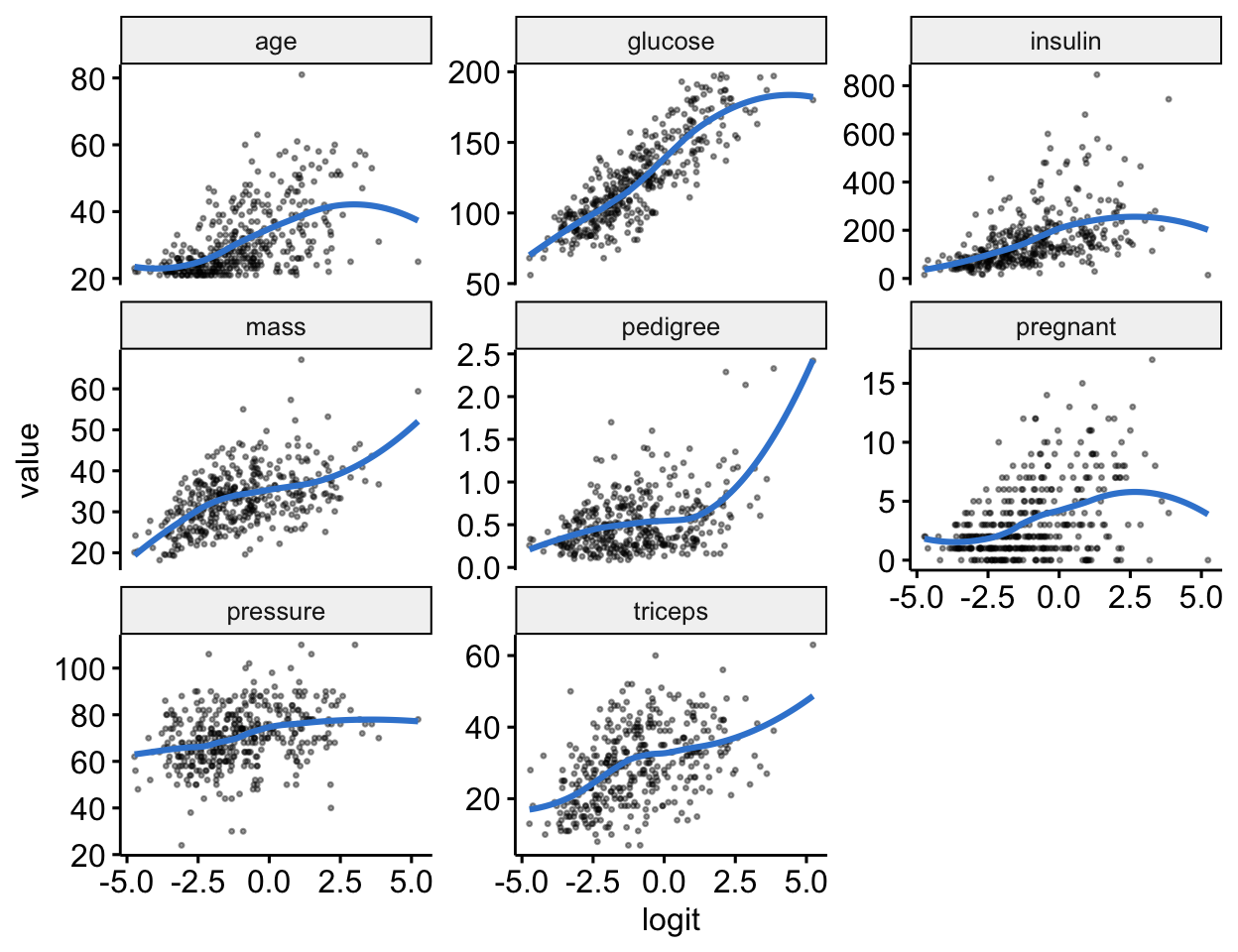
Logistic regression assumes each continuous predictor is linear against the logit (log-odds), not the probability. Compute the logit from the predicted probabilities and plot each predictor against it, with a loess smoother. We reshape to long form with base R (no tidyverse):
library(ggpubr)data("PimaIndiansDiabetes2", package ="mlbench")diabetes_data <-na.omit(PimaIndiansDiabetes2)model <-glm(diabetes ~ ., data = diabetes_data, family = binomial)probabilities <-predict(model, type ="response")# numeric predictors + the logit, reshaped long with base Rnum <- diabetes_data[sapply(diabetes_data, is.numeric)]logit <-log(probabilities / (1- probabilities))long <-data.frame(logit =rep(logit, ncol(num)),predictor =rep(names(num), each =nrow(num)),value =unlist(num))ggscatter(long, x ="logit", y ="value", size =0.5, alpha =0.4,add ="loess", add.params =list(color ="#3a86d4")) +facet_wrap(~ predictor, scales ="free_y")
Read each panel: a roughly straight loess curve means the predictor is linear in the logit. Here glucose, mass, pregnant, pressure, triceps look linear, while age and pedigree bend — they may need a transformation.
Tip
Verdict here: most predictors are linear in the logit; age and pedigree are not. If a predictor is non-linear, the fix is a non-linear term — log-transform it, add a polynomial (poly(x, 2)), or use a spline — then re-check the panel.
Influential values
Extreme points can distort the fit. Screen with Cook’s distance — plot(model, which = 4) labels the largest:
data("PimaIndiansDiabetes2", package ="mlbench")diabetes_data <-na.omit(PimaIndiansDiabetes2)model <-glm(diabetes ~ ., data = diabetes_data, family = binomial)plot(model, which =4, id.n =3)
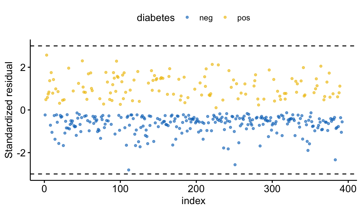
A large Cook’s distance only flags a point — it’s influential only if its standardized residual is also extreme (|value| > 3). Plot the standardized residuals by index, coloured by outcome:
library(ggpubr)data("PimaIndiansDiabetes2", package ="mlbench")diabetes_data <-na.omit(PimaIndiansDiabetes2)model <-glm(diabetes ~ ., data = diabetes_data, family = binomial)resid.df <-data.frame(index =seq_len(nrow(diabetes_data)),std_resid =rstandard(model),diabetes = diabetes_data$diabetes)ggscatter(resid.df, x ="index", y ="std_resid", color ="diabetes",palette ="jco", size =1, alpha =0.6,ylab ="Standardized residual") +geom_hline(yintercept =c(-3, 3), linetype ="dashed")
Tip
Verdict here: the largest standardized residual is ~2.8 — none exceeds ±3, so there are no influential outliers. If a point did exceed 3, options are: investigate it (data error?), remove the record, transform the predictor, or use a robust method.
Multicollinearity
Strongly correlated predictors make logistic coefficients unstable — the same VIF check as linear regression. car::vif(); anything above 5 is problematic:
library(car)data("PimaIndiansDiabetes2", package ="mlbench")diabetes_data <-na.omit(PimaIndiansDiabetes2)model <-glm(diabetes ~ ., data = diabetes_data, family = binomial)sort(vif(model), decreasing =TRUE)
     age pregnant     mass  triceps  insulin  glucose pressure pedigree
1.974053 1.892387 1.832416 1.638865 1.384038 1.378937 1.191287 1.031715
Tip
Verdict here: every VIF is well below 5 (the largest is ≈ 2) — no multicollinearity. If one exceeded 5, remove the redundant predictor (see multicollinearity & VIF).
Diagnosis summary
Assumption
Check
Good sign
Fix if violated
Binary outcome
the response
exactly two classes
use multinomial/ordinal models instead
Linearity of logit
predictor-vs-logit + loess
straight loess
transform / polynomial / spline the predictor
No influential points
Cook’s distance + std. residual
|std. resid| < 3
investigate / remove / transform
No multicollinearity
car::vif()
VIF < 5
remove the redundant predictor
Report
Logistic regression assumptions were checked. Most continuous predictors were linear in the logit (age and pedigree showed mild departures); no observations exceeded a standardized residual of 3 (no influential outliers); and all variance inflation factors were below 2 (no multicollinearity).
NoteThe math (optional)
The logit of the fitted probability is \(\text{logit}(p) = \log\!\dfrac{p}{1-p}\), which the model assumes is linear in each continuous predictor — that’s why you plot predictors against the logit, not the probability. The standardized (Pearson) residual rescales each raw residual by its standard error so extremes are comparable; Cook’s distance combines residual size and leverage to measure each point’s influence on the fit (same idea as in linear regression, adapted to the GLM). VIF is unchanged from linear regression — it’s computed on the predictor design matrix.
Try it live
Re-check the VIF after dropping a predictor, or inspect the logit-linearity for a single variable. The sandbox boots on first Run.
🟢 With an AI agent
Ask Prova“check the assumptions of my logistic regression and tell me which one is violated and how to fix it” — it inspects logit-linearity, influence and VIF, and answers with code you can run on your own model. The runtime is the judge.Ask Prova →
Common issues
You checked linearity against the probability, not the logit. Logistic regression assumes linearity in the log-odds — plot each continuous predictor against the logit, not the raw probability or the 0/1 outcome.
You treated a labelled Cook’s-distance point as an automatic outlier.plot(model, which = 4) labels the largest values, but a point is influential only if its standardized residual is also extreme (|value| > 3). Check both.
You forgot categorical predictors don’t need the linearity check. The logit-linearity assumption applies only to continuous predictors; factors are dummy-coded and exempt.
Frequently asked questions
NoteWhat are the assumptions of logistic regression?
Four: a binary outcome; a linear relationship between each continuous predictor and the logit (log-odds) of the outcome; no influential outliers; and no multicollinearity among predictors. (Logistic regression does not assume normality or homoscedasticity of residuals like linear regression.)
NoteHow do I check the linearity assumption in logistic regression?
Compute the logit of the fitted probabilities (log(p/(1-p))) and plot each continuous predictor against it with a loess smoother. A roughly straight loess curve means the predictor is linear in the logit; a clear bend means you should transform it (log, polynomial, or spline).
NoteHow do I find influential observations in a logistic regression?
Use plot(model, which = 4) for Cook’s distance to flag the largest values, then check the standardized residuals (rstandard(model)) — a point is a likely influential outlier only if its absolute standardized residual exceeds 3. Large Cook’s distance alone isn’t enough.
NoteDoes logistic regression assume normality of residuals?
No. Unlike linear regression, logistic regression does not assume normally distributed residuals or constant variance. Its assumptions are a binary outcome, linearity of the logit, no influential points, and no multicollinearity.
Test your understanding
ImportantPractice
Run it. In the live cell, check the VIFs. Are any predictors multicollinear (VIF > 5)?
Conceptual. A continuous predictor’s loess curve against the logit is strongly U-shaped. What does that tell you, and what’s one fix?
NoteHint
Compare each VIF to the rule-of-thumb threshold of 5. For question 2, recall that the linearity assumption is about the logit, and a curved relationship breaks it.
NoteSolution
All VIFs are below 2, so there is no multicollinearity to worry about. For question 2: a U-shaped loess curve means the predictor is not linear in the logit — the linearity assumption is violated. A fix is to add a quadratic term (poly(x, 2)) or a spline, which lets the model bend with the relationship; then re-plot to confirm the curve straightens.
Conclusion
You can now diagnose a logistic regression in R: confirm the binary outcome, check logit-linearity for each continuous predictor, screen for influential points with Cook’s distance and standardized residuals, and test multicollinearity with VIF — applying the right fix for any violation. A checked logistic model is one whose odds ratios you can report with confidence.
Every result on this page was produced by the code shown, run at build time against a pinned R environment — edit any block and Run to reproduce it yourself.