Predict in R: Model Predictions and Intervals

Use a fitted model to predict new outcomes with predict() — and report the right uncertainty: a confidence interval for the mean, a prediction interval for a single new case

Predict outcomes from a fitted regression in R with predict(). Make point predictions for new data, then show the uncertainty correctly — a confidence interval for the mean response versus a (wider) prediction interval for an individual new observation, and visualize both as bands.

TipKey takeaways

• Use predict(model, newdata) to estimate the outcome for new predictor values from a fitted model.
• A confidence interval (interval = "confidence") is the uncertainty around the mean outcome at those predictors — narrow.
• A prediction interval (interval = "prediction") is the uncertainty around a single new observation — wider, because it also includes individual scatter.
• Pass a data.frame whose column names match the model’s predictors.
• Plot both as bands around the fitted line to show the uncertainty visually.

Introduction

The point of a fitted regression is to predict — estimate the outcome for predictor values you haven’t seen. R’s predict() does this, and just as importantly tells you how uncertain the prediction is, in two different senses you must not confuse.

The scenario: from a model of car stopping distance vs speed, predict the stopping distance at new speeds — and report the right interval depending on whether you care about the average car or one specific car.

Build a model

We use the built-in cars dataset — speed (mph) and stopping distance (ft) for 50 cars — and fit a simple linear regression:

data("cars", package = "datasets")

model <- lm(dist ~ speed, data = cars)
model

Call:
lm(formula = dist ~ speed, data = cars)

Coefficients:
(Intercept)        speed  
    -17.579        3.932  

The equation is dist = -17.58 + 3.93 × speed — each extra mph adds ~3.9 ft of stopping distance.

Predict for new data

Build a data.frame of new predictor values (the column name must match the model’s predictor, speed), then call predict():

data("cars", package = "datasets")
model <- lm(dist ~ speed, data = cars)

new.speeds <- data.frame(speed = c(12, 19, 24))
predict(model, newdata = new.speeds)

       1        2        3 
29.60981 57.13667 76.79872 

A car at 19 mph is predicted to need ~57 ft to stop. These are point predictions — the best single guess, with no uncertainty attached yet.

Confidence interval — uncertainty of the mean

interval = "confidence" gives the interval for the mean outcome at each predictor value — “where the average stopping distance lies”:

data("cars", package = "datasets")
model <- lm(dist ~ speed, data = cars)
new.speeds <- data.frame(speed = c(12, 19, 24))

predict(model, newdata = new.speeds, interval = "confidence")

       fit      lwr      upr
1 29.60981 24.39514 34.82448
2 57.13667 51.82913 62.44421
3 76.79872 68.38765 85.20978

At 19 mph, the mean stopping distance is ~57 ft, 95% CI [51.8, 62.4] — a narrow band, because averages are estimated precisely.

Prediction interval — uncertainty of a single new case

interval = "prediction" gives the interval for one new individual observation — “where a single car’s stopping distance lies.” It is wider, because it adds the scatter of individual cars around the mean:

data("cars", package = "datasets")
model <- lm(dist ~ speed, data = cars)
new.speeds <- data.frame(speed = c(12, 19, 24))

predict(model, newdata = new.speeds, interval = "prediction")

       fit       lwr       upr
1 29.60981 -1.749529  60.96915
2 57.13667 25.761756  88.51159
3 76.79872 44.752478 108.84495

At 19 mph, a single car’s stopping distance has a 95% prediction interval of [25.8, 88.5] — far wider than the confidence interval, because individual cars vary a lot around the average. (Prediction intervals assume the residuals are roughly normal with constant variance — check the diagnostics before trusting them.)

Note

Confidence vs prediction — the one thing to get right. Confidence interval = uncertainty of the mean response (narrow). Prediction interval = uncertainty of a single future observation (wide). Same point estimate, different question, very different width.

Visualize both bands

Plot the fitted line with both bands — the narrow confidence band hugs the line, the wide prediction band captures most individual points:

library(ggpubr)

data("cars", package = "datasets")
model <- lm(dist ~ speed, data = cars)

# prediction interval for every observed speed
pred <- predict(model, interval = "prediction")
plot.df <- cbind(cars, pred)            # adds fit / lwr / upr columns

ggscatter(plot.df, x = "speed", y = "dist", color = "grey40",
          xlab = "Speed (mph)", ylab = "Stopping distance (ft)") +
  geom_ribbon(aes(ymin = lwr, ymax = upr), alpha = 0.15, fill = "#3a86d4") +
  geom_smooth(aes(y = dist), method = "lm", color = "#3a86d4", fill = "grey60")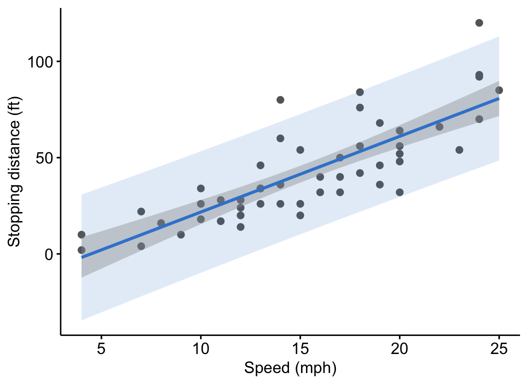

The inner (grey) band is the confidence interval for the mean; the outer (blue) band is the prediction interval for individual cars.

Report

Stopping distance was predicted from speed (dist = -17.6 + 3.93 × speed). At 19 mph the predicted mean stopping distance was 57 ft (95% CI 51.8–62.4), while the 95% prediction interval for a single car was much wider, 25.8–88.5 ft.

NoteThe math (optional)

Both intervals centre on the same fitted value \(\hat{y}_0 = \hat\beta_0 + \hat\beta_1 x_0\). The confidence interval uses the standard error of the mean response, \(\text{SE}_{\text{conf}} = s\sqrt{\tfrac{1}{n} + \tfrac{(x_0-\bar x)^2}{\sum (x_i-\bar x)^2}}\). The prediction interval adds the individual residual variance, \(\text{SE}_{\text{pred}} = s\sqrt{1 + \tfrac{1}{n} + \tfrac{(x_0-\bar x)^2}{\sum (x_i-\bar x)^2}}\) — the extra 1 under the root is the scatter of a single new point, which is why prediction intervals are always wider.

Try it live

Predict the stopping distance at a speed of your choice, with both intervals. The sandbox boots on first Run.

🟢 With an AI agent

Ask Prova “predict new values from my model and show the confidence and prediction intervals” — it answers with code you can run on your own fitted model and explains which interval to report. The runtime is the judge. Ask Prova →

Common issues

Your newdata column names don’t match the model. predict() needs a data.frame whose columns are named exactly like the model’s predictors (speed, not Speed or x). A mismatch silently predicts on the training data or errors.

You reported a confidence interval when you meant a prediction interval. If you’re predicting a single new outcome (one patient, one car), use interval = "prediction" — the confidence interval understates the uncertainty for an individual.

You predicted far outside the training range. predict() will happily extrapolate, but the model has no evidence out there — predictions (and intervals) beyond the observed predictor range are unreliable.

Frequently asked questions

NoteHow do I use predict() in R?

Fit the model with lm(), build a data.frame of new predictor values with the same column names as the model’s predictors, then call predict(model, newdata = new). Add interval = "confidence" or "prediction" to get the uncertainty around the prediction.

NoteWhat is the difference between a confidence interval and a prediction interval?

A confidence interval estimates the uncertainty of the mean outcome at given predictor values (narrow). A prediction interval estimates where a single new observation will fall (wider) — it adds the individual scatter around the mean. Same centre, different width; pick based on whether you care about the average or one new case.

NoteWhy is the prediction interval wider than the confidence interval?

Because it accounts for two sources of uncertainty: the uncertainty in estimating the mean (which the confidence interval also has) plus the natural variation of individual observations around that mean. That extra variance always makes the prediction interval wider.

Test your understanding

ImportantPractice

1. Run it. In the live cell, predict the stopping distance at 30 mph with both intervals. How much wider is the prediction interval than the confidence interval?
2. Conceptual. You want to tell a single driver how far their specific car will take to stop at 30 mph. Which interval do you quote, and why?

NoteHint

Fill the blank with "confidence", then "prediction", and compare the widths. For question 2, think about whether the driver cares about the average car or their car.

NoteSolution

The prediction interval is much wider (it includes individual-car scatter). For question 2: quote the prediction interval — the driver is asking about one specific car, a single new observation, so the confidence interval (which only describes the mean car) would badly understate the real uncertainty.

Conclusion

You can now predict in R with predict(): make point predictions for new data, and report the right uncertainty — a confidence interval for the mean response, a prediction interval for a single new observation — and visualize both as bands. Getting the two intervals straight is the difference between an honest prediction and an overconfident one.

Related lessons

• Simple linear regression in R · Multiple linear regression in R — fit the models you predict from. · Linear regression assumptions & diagnostics in R — make sure the model (and its intervals) are trustworthy first.
• Go further: Regression analysis · Biostatistics

Was this page helpful?

Prove you can do it. Master the whole Regression in R series — track your path, build projects, and earn a certificate.

Start free →

Go Pro — unlimited Prova on your own data and a verifiable certificate that proves the skill.

from $15/mo billed yearly

Go Pro →

✓ You're Pro — keep going. The runtime is the judge.

Ready to level up?

Try this on your own data with Prova — the runtime is the judge.Open Prova →

Get new R & Python lessons by email

Practical, reproducible, no spam. Unsubscribe anytime.

Double opt-in. We never share your email.

Share this pageXLinkedInRedditHN

Note

Every result on this page was produced by the code shown, run at build time against a pinned R environment — edit any block and Run to reproduce it yourself.