Frailty Models in R: Mixed-Effects Cox for Clustered Survival Data (coxme)

Patients within centers, recurrent events within a subject, litter-matched animals — add a random effect (the frailty) to a Cox model with coxme so your standard errors stop assuming independence that isn’t there

Fit a frailty (mixed-effects / random-effects Cox) model in R with the coxme package. When survival times are clustered or correlated — patients within hospitals, repeated events within one patient, litters of animals — a shared frailty adds a random effect per cluster so the model accounts for the within-cluster correlation. Fit a shared-frailty model with coxme, interpret the fixed-effect hazard ratios and the frailty variance, compare with a naive coxph, see the older coxph(frailty()) route, test whether the random effect matters, and plot the per-cluster random effects.

TipKey takeaways

• When survival times are clustered, a plain Cox model is wrong — patients in the same hospital, repeated events within one patient, or litter-matched animals are correlated, and coxph() assumes they are independent. That assumption deflates the standard errors and overstates precision.
• A frailty is a shared, unobserved random effect — one multiplicative term on the hazard per cluster — that soaks up the between-cluster variation the fixed covariates don’t explain.
• Fit it with coxme() from the coxme package: a random intercept per cluster is (1 | cluster). coxme(Surv(time, status) ~ rx + (1 | litter), data) reads exactly like lme4.
• Interpret two things: the fixed-effect hazard ratios (exp(fixef()), adjusted for clustering) and the frailty variance (VarCorr()) — how much baseline risk varies between clusters.
• The older coxph(... + frailty(id, distribution = "gamma")) route still works; coxme is the modern mixed-model approach and the one to reach for now.
• Test whether the random effect matters with a likelihood-ratio test against the no-frailty Cox model, and see the clusters with a caterpillar plot of the per-cluster random effects (ranef()).

Introduction

You are analyzing a 100-litter rat carcinogenesis study, or a 37-center oncology trial, or a kidney-catheter dataset where each patient contributes two infection times. In every one of these, the survival times are not independent — rats from the same litter share genetics and a cage, patients in the same hospital share a standard of care and case-mix, two events from the same patient share that patient. Feed this to a plain Cox model and you get a tidy hazard ratio with a standard error that is too small: coxph() counts every observation as fresh information, so it overstates how much you really know.

The fix is a frailty — a random effect added to the Cox model, one per cluster. Each cluster gets its own unobserved multiplier on the baseline hazard: a “high-frailty” litter dies faster across the board, a “low-frailty” center has better baseline survival, for reasons your covariates never measured. The model estimates how much that hidden multiplier varies (the frailty variance) and corrects the fixed-effect inference for the within-cluster correlation. It is the survival-analysis twin of a mixed-effects model: fixed effects for the covariates you care about, a random intercept for the cluster.

This lesson fits frailty models in R with coxme (Therneau’s mixed-effects Cox package) and the base survival package, on litter-matched and multi-center data. You will learn to:

• recognize when clustering breaks a plain Cox model;
• fit a shared-frailty model with coxme() and the (1 | cluster) syntax;
• interpret the fixed-effect HRs and the frailty variance;
• compare it with a naive coxph() and see the standard errors change;
• use the older coxph(frailty()) route and know why coxme superseded it;
• test whether the random effect matters and plot the per-cluster effects.

NoteWhat a frailty adds to the Cox model

A standard Cox model gives every subject the same baseline hazard \(h_0(t)\). A shared-frailty model multiplies it by a cluster-specific random term \(u_i\) (the frailty), shared by everyone in cluster \(i\):

\[ h_{ij}(t) = h_0(t)\, u_i \,\exp(b_1 x_{1ij} + \dots + b_p x_{pij}) \]

Equivalently, on the log scale, each cluster has a random intercept \(w_i = \log u_i \sim N(0, \sigma^2)\). The model estimates the fixed coefficients \(b\) and the frailty variance \(\sigma^2\). A larger \(\sigma^2\) means clusters differ more in baseline risk; \(\sigma^2 = 0\) collapses back to an ordinary Cox model.

The data: a litter-matched rat study

We use rats, the classic litter-matched tumorigenesis experiment that ships with the survival package. Each of 100 litters has three rats — one given a drug (rx = 1) and two controls (rx = 0) — and we record time to tumor. Litter is the cluster: rats from the same litter share genetics, so their tumor times are correlated. rats is part of the survival package’s lazy-loaded data, so just reference it after library(survival):

library(survival)

head(rats)

  litter rx time status sex
1      1  1  101      0   f
2      1  0   49      1   f
3      1  0  104      0   f
4      2  1   91      0   m
5      2  0  104      0   m
6      2  0  102      0   m

c(rats = nrow(rats), litters = length(unique(rats$litter)), tumors = sum(rats$status))

   rats litters  tumors 
    300     100      42 

The columns we model:

• time / status — time to tumor and the event indicator (1 = tumor, 0 = censored).
• rx — the treatment: 1 = drug, 0 = control. This is the fixed effect we want a hazard ratio for.
• litter — the cluster (1–100), three rats each. This becomes the random effect.

Only 42 of 300 rats developed a tumor — a heavily censored dataset, typical of survival data.

Why clustering matters: the naive Cox model first

Start with the model that ignores the litters, so you have a baseline to compare against. Fit a plain Cox model of tumor time on treatment:

library(survival)

naive <- coxph(Surv(time, status) ~ rx, data = rats)
summary(naive)$coefficients

        coef exp(coef)  se(coef)       z   Pr(>|z|)
rx 0.7137368  2.041606 0.3087778 2.31149 0.02080582

Read it: the drug raises the hazard of tumor — exp(coef) ≈ 2.04, so treated rats develop tumors at about twice the rate of controls (HR = 2.04, p = 0.021). The standard error of the log-HR is 0.309. That number is the problem: it treats all 300 rats as independent, when really there are only 100 independent litters. Ignoring the litter correlation makes the SE too small and the result look more certain than it is. We need a model that knows three rats share a litter.

Fit the shared-frailty model with coxme()

The modern tool is coxme() from the coxme package. Its formula reads exactly like lme4: fixed effects on the left, a random intercept for the cluster as (1 | litter). That (1 | litter) is the shared frailty — one random multiplier on the hazard per litter:

library(survival)
library(coxme)

fit <- coxme(Surv(time, status) ~ rx + (1 | litter), data = rats)
fit

Cox mixed-effects model fit by maximum likelihood
  Data: rats
  events, n = 42, 300
  Iterations= 19 81 
                    NULL Integrated    Fitted
Log-likelihood -225.2822  -218.4886 -183.0781

                  Chisq   df          p   AIC    BIC
Integrated loglik 13.59  2.0 1.1210e-03  9.59   6.11
 Penalized loglik 84.41 33.4 2.6679e-06 17.61 -40.43

Model:  Surv(time, status) ~ rx + (1 | litter) 
Fixed coefficients
        coef exp(coef)  se(coef)   z     p
rx 0.7301151  2.075319 0.3177679 2.3 0.022

Random effects
 Group  Variable  Std Dev  Variance
 litter Intercept 1.147775 1.317388

Interpret the output in plain language — there are two parts:

• Fixed effects — the part you report like an ordinary Cox model. rx: coef = 0.730, HR = exp(0.730) ≈ 2.08, p = 0.022. Adjusted for the litter clustering, the drug still roughly doubles the tumor hazard. Note the standard error: 0.318, slightly larger than the naive 0.309 — the frailty has widened it to honestly reflect the 100 (not 300) independent units. (The correction is modest here because the design is balanced and most litters are censored; with more events per cluster it grows.)
• Random effects — the new piece. The frailty variance for litter is Variance = 1.32 (Std Dev = 1.15 on the log-hazard scale). That is large: litters differ a lot in baseline tumor risk for reasons rx doesn’t capture. A frailty SD of 1.15 means a litter one SD above average has a baseline hazard exp(1.15) ≈ 3.2× that of an average litter. The clustering is real and worth modelling.
• The likelihood-ratio test at the top (Integrated loglik χ² = 13.6 on 2 df, p = 0.001) confirms the model as a whole — fixed effect plus frailty — beats the null.

Pull the pieces out directly when you need them:

library(survival)
library(coxme)

fit <- coxme(Surv(time, status) ~ rx + (1 | litter), data = rats)

# Fixed-effect hazard ratio
exp(fixef(fit))

      rx 
2.075319 

# The frailty variance (between-litter variance on the log-hazard scale)
VarCorr(fit)

$litter
Intercept 
 1.317388 

Does the random effect matter? A likelihood-ratio test

A frailty variance of 1.32 looks large, but test it: compare the frailty model against the plain Cox model with no frailty with a likelihood-ratio test. Twice the gap in log-likelihood is a χ² statistic; because you are testing a variance on the boundary (σ² = 0), use a ½ χ²₁ reference (a standard mixed-model correction):

library(survival)
library(coxme)

no.frailty <- coxph(Surv(time, status) ~ rx, data = rats)               # σ² = 0
with.frailty <- coxme(Surv(time, status) ~ rx + (1 | litter), data = rats)

lrt <- 2 * (with.frailty$loglik["Integrated"] - as.numeric(logLik(no.frailty)))
p.value <- 0.5 * pchisq(lrt, df = 1, lower.tail = FALSE)                 # boundary correction
c(chisq = round(lrt, 2), p = signif(p.value, 3))

chisq.Integrated     p.Integrated 
         8.35000          0.00192 

Read it: χ² ≈ 8.35, p ≈ 0.002. The random effect is highly significant — adding the litter frailty improves the model substantially, so the litters genuinely differ in baseline risk and you should keep the frailty. If this test were non-significant, a plain coxph() would be adequate and you could drop the random effect.

The older route: coxph(... + frailty())

Before coxme, the survival package fit frailty models through a frailty() term inside coxph(). It still works and you will meet it in older code, so know it:

library(survival)

fit.old <- coxph(Surv(time, status) ~ rx + frailty(litter, distribution = "gamma"), data = rats)
fit.old

Call:
coxph(formula = Surv(time, status) ~ rx + frailty(litter, distribution = "gamma"), 
    data = rats)

                            coef se(coef)    se2  Chisq   DF     p
rx                         0.727    0.318  0.313  5.219  1.0 0.022
frailty(litter, distribut                        63.046 47.7 0.067

Iterations: 6 outer, 23 Newton-Raphson
     Variance of random effect= 2.02   I-likelihood = -217.5 
Degrees of freedom for terms=  1.0 47.7 
Likelihood ratio test=88.5  on 48.6 df, p=4e-04
n= 300, number of events= 42 

Read it: the rx coefficient (0.727, HR ≈ 2.07, p = 0.022) matches the coxme fit closely, and the variance of the random effect is 2.02 — a different number because this uses a gamma frailty (multiplicative on the hazard) rather than coxme’s log-normal random effect (a normal random intercept). Both describe the same between-litter variation on different scales; the conclusion — substantial clustering, a drug HR near 2 — is the same.

NoteWhy prefer coxme now?

coxph(frailty()) is a penalized-likelihood approximation that Therneau himself considers superseded. coxme fits the random effect by a proper mixed-model (integrated) likelihood, generalizes cleanly to multiple and crossed random effects and random slopes ((rx | center)), and reads like the rest of the lme4 mixed-model world. Use coxme for new work; recognize coxph(frailty()) in legacy code.

The signature figure: per-cluster random effects (a caterpillar plot)

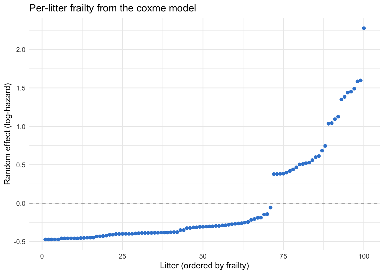
A frailty model gives you a predicted random effect — a BLUP (best linear unbiased predictor) — for every cluster: how much that litter’s baseline risk sits above or below average. Pull them with ranef() and draw a caterpillar plot (the random-effects equivalent of a forest plot), ordered from lowest to highest frailty. ggforest() does not support coxme, so build it directly in ggplot2:

library(survival)
library(coxme)
library(ggplot2)

fit <- coxme(Surv(time, status) ~ rx + (1 | litter), data = rats)

# Extract the per-litter random effects (BLUPs) and order them
re <- ranef(fit)$litter
df <- data.frame(litter = names(re), frailty = as.numeric(re))
df <- df[order(df$frailty), ]
df$rank <- seq_len(nrow(df))

ggplot(df, aes(x = rank, y = frailty)) +
  geom_hline(yintercept = 0, linetype = "dashed", colour = "grey50") +
  geom_point(colour = "#3a86d4", size = 1.6) +
  labs(x = "Litter (ordered by frailty)", y = "Random effect (log-hazard)",
       title = "Per-litter frailty from the coxme model") +
  theme_minimal()

Read it: each point is one litter’s random effect on the log-hazard scale. Litters on the right (positive) have higher baseline tumor risk than average; litters on the left (negative) are protected. The spread — most litters within about ±0.5, with a few markedly higher — is the frailty variance made visible: substantial between-litter variation that a plain Cox model would have lumped into the error. This is the picture that shows a reviewer why you needed the frailty.

Recurrent events: a per-subject frailty for repeated events

Frailty isn’t only for groups of subjects — it also models repeated events within one subject. When a patient can have the same event more than once (recurrent infections, hospital readmissions), the events from one patient are correlated, and the patient is the cluster. A per-subject frailty handles it:

library(survival)
library(coxme)

# kidney: time to catheter infection, up to 2 events per patient (id = the cluster)
fit.k <- coxme(Surv(time, status) ~ age + sex + (1 | id), data = kidney)
fit.k

Cox mixed-effects model fit by maximum likelihood
  Data: kidney
  events, n = 58, 76
  Iterations= 6 34 
                    NULL Integrated    Fitted
Log-likelihood -187.9028  -181.9045 -166.1653

                  Chisq    df          p   AIC    BIC
Integrated loglik 12.00  3.00 0.00739530  6.00  -0.18
 Penalized loglik 43.48 14.75 0.00011458 13.97 -16.43

Model:  Surv(time, status) ~ age + sex + (1 | id) 
Fixed coefficients
          coef exp(coef)   se(coef)     z      p
age  0.0042892 1.0042984 0.01171041  0.37 0.7100
sex -1.3549853 0.2579511 0.41712539 -3.25 0.0012

Random effects
 Group Variable  Std Dev   Variance 
 id    Intercept 0.6754474 0.4562292

Read it: kidney records up to two catheter-infection times per patient, so id is the cluster. The fixed effects (age, sex) are adjusted for the per-patient frailty, and the frailty variance measures how much patients differ in their underlying infection rate — sex shows a strong protective effect for women (HR well below 1). For the counting-process layout that recurrent-event data often needs (one row per at-risk interval, Surv(start, stop, status)), see time-varying covariates; a per-subject frailty layers on top of it the same way.

TipClustered vs recurrent — same tool, two shapes

• Clustered data (patients in centers, rats in litters): many subjects per cluster, one event each → a shared frailty per cluster, (1 | center).
• Recurrent events (repeated infections within a patient): one subject, many events → a per-subject frailty, (1 | id), usually on a counting-process Surv(start, stop, status) layout.

A clinical framing: a multi-center trial

The same machinery gives the canonical clinical use — a multi-center trial where institution is a random effect. The coxme package ships the eortc dataset for exactly this: a simulated bladder-cancer trial across 37 centers. Because eortc lives in the coxme package (not the survival package), it is not lazy-loaded — load it explicitly with data(eortc):

library(survival)
library(coxme)
data(eortc)                       # lives in coxme, so data() IS needed here

fit.e <- coxme(Surv(y, uncens) ~ trt + (1 | center), data = eortc)
fit.e

Cox mixed-effects model fit by maximum likelihood
  Data: eortc
  events, n = 1463, 2323
  Iterations= 9 49 
                    NULL Integrated    Fitted
Log-likelihood -10638.71  -10520.65 -10478.84

                   Chisq    df p    AIC    BIC
Integrated loglik 236.11  2.00 0 232.11 221.53
 Penalized loglik 319.74 28.69 0 262.37 110.67

Model:  Surv(y, uncens) ~ trt + (1 | center) 
Fixed coefficients
         coef exp(coef)   se(coef)     z p
trt 0.7086127  2.031171 0.06424398 11.03 0

Random effects
 Group  Variable  Std Dev   Variance 
 center Intercept 0.3292140 0.1083818

Read it: across 37 centers, treatment carries HR = exp(0.709) ≈ 2.03 (p < 0.001), and the center frailty variance is 0.108 (SD ≈ 0.33) — centers differ modestly in baseline hazard. Compare the treatment SE to a naive coxph(Surv(y, uncens) ~ trt) (SE ≈ 0.063 either way here, because with 1463 events the center variance is small): the frailty matters most when between-cluster variance is large relative to the within-cluster information. Reporting the center frailty also tells your readers the treatment effect is consistent across institutions, not driven by one site.

Report

Because the rats were litter-matched, tumor times within a litter are correlated, so we fitted a shared-frailty (mixed-effects) Cox model with a random intercept per litter using the coxme package. The treatment was associated with a higher hazard of tumor (HR = 2.08, 95% CI 1.11–3.87, p = 0.022), adjusted for between-litter variation. The estimated litter frailty variance was 1.32 (SD = 1.15 on the log-hazard scale), and a likelihood-ratio test confirmed the random effect was needed (χ² = 8.35, p = 0.002), indicating substantial heterogeneity in baseline risk across litters that a standard Cox model would have ignored.

NoteThe math behind the frailty (optional)

Write each cluster’s random intercept as \(w_i \sim N(0, \sigma^2)\), so the frailty multiplier is \(u_i = \exp(w_i)\) (log-normal, the coxme default). The hazard for subject \(j\) in cluster \(i\) is:

\[ h_{ij}(t) = h_0(t)\,\exp\!\big(x_{ij}^\top b + w_i\big) \]

Because the \(w_i\) are unobserved, coxme integrates them out of the partial likelihood to get a marginal (integrated) likelihood in \(b\) and \(\sigma^2\), then maximizes it — the same logic as a generalized linear mixed model. The estimated \(\hat\sigma^2\) is the frailty variance you read off VarCorr(); the predicted \(\hat w_i\) are the BLUPs from ranef() you plotted. The older coxph(frailty(..., distribution = "gamma")) instead takes \(u_i \sim \text{Gamma}(1/\theta, 1/\theta)\) and fits \(\theta\) by penalized likelihood — a different distribution and estimator for the same idea, which is why its variance (2.02) is on a different scale from coxme’s 1.32.

Frailty or stratification? Which to reach for

A frailty and a stratified Cox model both handle a categorical clustering variable, but they answer different questions:

TipChoosing how to handle a clustering variable

• You want to estimate the between-cluster variation and treat clusters as a sample from a population (generalize beyond these 37 centers / 100 litters) → a frailty ((1 | cluster)). It costs one parameter (the variance) and gives an honest, correlation-adjusted fixed-effect SE.
• You only need to control for the cluster as a nuisance, with no interest in its variation, and you have few clusters with many events each → stratify it (strata(cluster)) — each cluster its own baseline, no variance assumption. See stratified Cox.
• The cluster’s effect changes over time (it violates proportional hazards) → stratification or a time-varying term, not a frailty (the frailty assumes a constant multiplier).
• Rule of thumb: many clusters → frailty (you can estimate the variance); few clusters → stratify (a variance from 3 clusters is unreliable).

Try it live

Fit a frailty model yourself — change the dataset, swap the cluster, or compare the fixed-effect SE against a naive coxph(). The sandbox boots on first Run (it downloads survival + coxme, so give it a moment).

🟢 With an AI agent

Ask Prova “my survival data is clustered — patients within hospitals — fit a shared-frailty mixed-effects Cox model with coxme, show me the hazard ratios and the frailty variance, and tell me whether the random effect is needed” — it answers with survival + coxme code you can run on your own data. The runtime is the judge. Ask Prova →

Common issues

You ignored the clustering and trusted the naive coxph() standard errors. This is the whole reason frailty models exist: when subjects are correlated (same center, same patient, same litter), coxph() counts each as independent and reports a standard error that is too small, so confidence intervals are too narrow and p-values too optimistic. If your design has a natural grouping, model it — either a frailty (coxme) or, if you only need a robust SE without estimating the variance, coxph(..., cluster = id) for a sandwich (robust) variance.

You confused frailty with stratification. They are not interchangeable. A frailty estimates the between-cluster variance and treats clusters as a random sample — use it with many clusters when you care about the variation and want to generalize. Stratification gives each cluster its own baseline and estimates nothing about it — use it with few clusters that are nuisance confounders. A variance estimated from 3 centers is meaningless; a frailty from 100 litters is informative.

The model won’t converge, or the variance pins at zero. Too few clusters, or too few events per cluster, leaves nothing for the random effect to estimate — coxme may report a near-zero variance or fail to converge. You need a reasonable number of clusters (a rough floor of ~5–10, comfortable with ≥ 20) and some events spread across them. With too few clusters, stratify instead, or drop the random effect if a likelihood-ratio test says it isn’t needed.

Frequently asked questions

NoteWhat is a frailty model in survival analysis?

A frailty model is a Cox model with a random effect (the frailty) added for clustered or correlated survival times. Each cluster — a hospital, a patient with recurrent events, a litter — gets its own unobserved multiplier on the baseline hazard, shared by everyone in the cluster. It is the survival-data version of a mixed-effects model: fixed effects for your covariates, a random intercept for the cluster. Fit it in R with coxme(Surv(time, status) ~ x + (1 | cluster), data).

NoteHow do I fit a mixed-effects Cox model in R?

Use the coxme package. The syntax mirrors lme4: coxme(Surv(time, status) ~ rx + (1 | center), data), where (1 | center) is a random intercept (a shared frailty) per center. Read the fixed effects like an ordinary Cox model (exp(fixef(fit)) for hazard ratios) and the frailty variance from VarCorr(fit). The older coxph(... + frailty(center, distribution = "gamma")) route also works, but coxme is the modern mixed-model approach.

NoteWhat is the difference between a frailty model and a stratified Cox model?

A frailty treats the clustering variable as a random effect — it estimates the variance of baseline risk across clusters and assumes clusters are a sample from a population, so you can generalize beyond them. Stratification (strata()) gives each cluster its own baseline but estimates nothing about it, treating the cluster as a fixed nuisance. Reach for a frailty when you have many clusters and care about the between-cluster variation; stratify when you have few clusters that are just confounders.

NoteHow do I interpret the frailty variance?

The frailty variance (from VarCorr()) is the variance of the random intercept on the log-hazard scale — how much baseline risk varies between clusters after accounting for your covariates. Take its square root for the standard deviation: a cluster one SD above average has baseline hazard exp(SD) times the average. A large variance means clusters differ a lot (the frailty is doing real work); a variance near zero means clustering is negligible and a plain Cox model would do.

NoteHow many clusters do I need to fit a frailty model?

Enough to estimate a variance reliably — a variance computed from 3 or 4 clusters is meaningless. A rough floor is around 5–10 clusters, and you are comfortable with 20 or more, ideally with several events spread across them. With too few clusters (or too few events per cluster), coxme may fail to converge or pin the frailty variance at zero; in that case stratify on the variable instead, or drop the random effect if a likelihood-ratio test shows it isn’t needed.

Test your understanding

ImportantPractice

1. Run it. In the live cell below, fit a shared-frailty model on the rats data, then fit the naive coxph() that ignores the litters. Fill the blank. Compare the standard error of rx between the two models — which is larger, and why?
2. Interpret. A frailty model reports a litter frailty variance of 0.02 (SD ≈ 0.14) and a likelihood-ratio test for the random effect with p = 0.61. Is the clustering worth modelling here? What would you do instead?

NoteHint

Fill the blank with litter — the cluster. (1 | litter) is the shared frailty. Compare se(coef) for rx in the coxme Fixed coefficients block against se(coef) in the naive summary() output; the frailty widens it to account for the 100 (not 300) independent units.

NoteSolution

fit  <- coxme(Surv(time, status) ~ rx + (1 | litter), data = rats)
fit
#> Fixed effect rx: coef 0.730, HR 2.08, se 0.318, p 0.022
#> Random effect: litter variance 1.32 (SD 1.15)

naive <- coxph(Surv(time, status) ~ rx, data = rats)
summary(naive)$coefficients
#> rx: coef 0.714, HR 2.04, se 0.309, p 0.021

The coxme standard error (0.318) is larger than the naive one (0.309). The frailty model knows the 300 rats come from only 100 independent litters, so it widens the SE to reflect that — the naive model’s smaller SE overstates precision by treating correlated rats as independent.

For question 2: no, a frailty variance of 0.02 with a non-significant likelihood-ratio test (p = 0.61) means the clusters barely differ in baseline risk — the random effect is not needed. Drop it and fit a plain coxph(); the simpler model is adequate and the litters add nothing.

TipQuick check

You fit coxme(Surv(time, status) ~ trt + (1 | hospital), data) on a 40-hospital trial and get a frailty variance of 0.45 (SD ≈ 0.67) with a likelihood-ratio test p = 0.003. What does this tell you, and how do you report the treatment effect?

NoteShow answer

Hospitals differ substantially in baseline risk (frailty SD 0.67 → a hospital one SD above average has ~exp(0.67) ≈ 2× the baseline hazard), and the significant likelihood-ratio test (p = 0.003) confirms the random effect is needed — modelling the clustering was the right call. Report the fixed-effect treatment hazard ratio (exp(fixef(fit))) with its now-correctly-widened 95% CI, plus the frailty variance to document the between-hospital heterogeneity, noting the treatment effect is estimated across hospitals rather than driven by any single site.

Conclusion

You can now fit a frailty (mixed-effects Cox) model in R for clustered or correlated survival data. When subjects share a cluster — patients in a center, recurrent events in one patient, rats in a litter — a plain coxph() assumes an independence that isn’t there and reports standard errors that are too small. coxme() adds a random intercept per cluster, (1 | cluster), that absorbs the between-cluster variation: you read the fixed-effect hazard ratios like an ordinary Cox model and the frailty variance that quantifies how much baseline risk varies between clusters. On the litter-matched rats, the drug roughly doubled the tumor hazard (HR = 2.08) while the litters differed substantially in baseline risk (frailty variance 1.32, LRT p = 0.002). You compared it with the naive model, met the older coxph(frailty()) route, tested whether the random effect mattered, and plotted the per-cluster frailties. Reach for a frailty when you have many clusters and want to model their variation; stratify when you have few nuisance clusters instead.

Related lessons

• Stratified Cox model — the other way to handle a categorical clustering variable (few clusters, nuisance confounder), and when to prefer it over a frailty. · Time-varying covariates — the counting-process layout that recurrent-event frailty models sit on top of. · Cox proportional hazards model — the base model the frailty extends, with its hazard ratios and forest plot. · Competing risks — the other extension for non-standard survival data, when subjects can fail from more than one cause.
• Go further: Survival Analysis — the full series. · Biostatistics — the pillar.

Was this page helpful?

Prove you can do it. Master the whole Survival Analysis in R series — track your path, build projects, and earn a certificate.

Start free →

Go Pro — unlimited Prova on your own data and a verifiable certificate that proves the skill.

from $15/mo billed yearly

Go Pro →

✓ You're Pro — keep going. The runtime is the judge.

Ready to level up?

Try this on your own data with Prova — the runtime is the judge.Open Prova →

Get new R & Python lessons by email

Practical, reproducible, no spam. Unsubscribe anytime.

Double opt-in. We never share your email.

Share this pageXLinkedInRedditHN

Note

Every result on this page was produced by the code shown, run at build time against a pinned R environment — edit any block and Run to reproduce it yourself.