CDISC ADTTE in R: Submission-Grade Survival Analysis, Step by Step
Take a time-to-event endpoint from a CDISC ADaM ADTTE dataset through a submission-style analysis in R — the CNSR censoring flip, KM with median + 95% CI, the stratified log-rank test, the primary Cox hazard ratio, and a CSR-style gtsummary table
Biostatistics
Analyze a clinical-trial time-to-event endpoint the regulatory way in R. Map a CDISC ADaM ADTTE dataset to a Surv() object — handling the CNSR convention where 1 means censored (the opposite of R’s status), build event = 1 - CNSR, then run the submission analysis set: a Kaplan-Meier curve with risk table, median overall survival with its 95% confidence interval, the stratified log-rank test, the primary Cox hazard ratio with 95% CI, a proportional-hazards check, and a CSR-style summary table with gtsummary — framed by ICH E9(R1) estimand thinking.
Published
June 26, 2026
Modified
July 7, 2026
TipKey takeaways
A CDISC ADaM ADTTE dataset is the analysis-ready contract for a time-to-event endpoint: one record per subject per parameter (PARAMCD = OS, PFS, …), with the time in AVAL, the units in AVALU, and the censoring flag in CNSR.
The #1 mistake — the censoring flip. CDISC codes CNSR = 1 as censored and CNSR = 0 as the event — the opposite of R’s Surv(time, event), which wants event = 1. Always build event = 1 - CNSR before you model. Get this backwards and every result is silently wrong.
Run the submission analysis set on Surv(AVAL, 1 - CNSR): a Kaplan-Meier curve (risk table + CI + median lines), median OS with 95% CI per arm, the stratified log-rank test, and the Cox hazard ratio with 95% CI — the primary estimand.
On a CDISC-shaped adjuvant colon-cancer trial, Lev+5FU cut the hazard of death by ~30% (HR = 0.70, 95% CI 0.55–0.88, p = 0.003), with the proportional-hazards assumption holding (p = 0.34).
Summarize it the way a clinical study report does — a gtsummary median + survival-probability table and a tbl_regression of the Cox HR — and frame it with ICH E9(R1) estimand thinking: pre-specified endpoint, censoring rules, and stratification factors.
Introduction
You have been handed an ADTTE dataset for a clinical study report. The protocol’s primary endpoint is overall survival; the statistician before you mapped the raw data to CDISC ADaM standards, and now it is your job to produce the time-to-event analysis the submission needs — a Kaplan-Meier curve, median survival with confidence intervals, the log-rank test, and the primary hazard ratio.
If you have run a Cox model on the lung data, you already know the statistics. What changes in a regulatory setting is the data contract and the rigor around it. Two things bite people first:
ADTTE structure — survival data arrives in a fixed shape (one row per subject per parameter) with fixed variable names. You don’t get to pick columns; you map to them.
The censoring convention is flipped. CDISC’s CNSR flag uses 1 = censored, whereas R’s Surv(time, event) wants event = 1 for the event. Mix these up and your hazard ratio points the wrong way — a silent, catastrophic error a reviewer will catch.
This lesson takes a CDISC-shaped ADTTE dataset through a submission-style analysis in R with survival (the engine), survminer (the publication-grade KM plot), and gtsummary (the CSR-style tables). It is the bridge from “I can fit a Cox model” to “I can produce a submission-grade time-to-event analysis.”
What an ADTTE dataset is — and why the structure matters
ADTTE is the ADaM (Analysis Data Model) standard for time-to-event analysis. The discipline that makes it submission-ready is one rule: one record per subject per analysis parameter. A subject with two endpoints — overall survival (OS) and progression-free survival (PFS) — has two ADTTE rows, one per PARAMCD. You analyze one parameter at a time by filtering on PARAMCD.
These are the ADTTE variables that drive a survival analysis:
Variable
Meaning
Example
STUDYID
Study identifier
COLON-ADJ-001
USUBJID
Unique subject identifier
COLON-ADJ-001-0042
PARAMCD / PARAM
Parameter code / label
OS / Overall Survival
AVAL
Analysis value = time to event or censoring
2083
AVALU
Analysis value unit
DAYS
CNSR
Censoring flag — 0 = event, 1 = censored
0
EVNTDESC
Event description
Death
CNSDTDESC
Censoring-date description
Last known alive
TRT01P
Planned treatment (arm)
Lev+5FU
STARTDT / ADT
Time origin / analysis date
2021-03-14
The analysis value is already derived: AVAL is the time from the protocol-defined origin (STARTDT, e.g. randomization) to the analysis date (ADT, the event or the censoring date). Your job is not to re-derive time — it is to map AVAL, CNSR, and TRT01P into Surv() correctly and run the pre-specified analysis.
Build the ADTTE dataset (the mapping, made explicit)
Real ADTTE data is confidential, so here we derive a CDISC-shaped ADTTE dataset from the public colon dataset that ships with the survival package — an adjuvant therapy trial in colon cancer. Building it by hand is the point: it shows you the exact mapping you’ll apply to the real thing.
colon has two rows per subject (recurrence and death events, in etype). We take the death records (etype == 2) as the overall-survival parameter, and two arms — Observation vs Lev+5FU (the active adjuvant regimen):
library(survival)# Overall-survival records (death endpoint), two armsos <-subset(colon, etype ==2& rx %in%c("Obs", "Lev+5FU"))os$rx <-droplevels(os$rx)# Map raw trial data to a CDISC ADaM ADTTE structureadtte <-data.frame(STUDYID ="COLON-ADJ-001",USUBJID =sprintf("COLON-ADJ-001-%04d", os$id),PARAMCD ="OS",PARAM ="Overall Survival (days)",AVAL = os$time, # time to event / censoringAVALU ="DAYS",CNSR =1- os$status, # CDISC: 1 = censored, 0 = eventEVNTDESC =ifelse(os$status ==1, "Death", "Censored: alive at last follow-up"),TRT01P =factor(os$rx, levels =c("Obs", "Lev+5FU"),labels =c("Observation", "Lev+5FU")),STRAT =factor(ifelse(os$differ ==3, "Poor", "Well/Moderate")), # stratification factorstringsAsFactors =FALSE)adtte <- adtte[!is.na(adtte$STRAT), ] # drop unknown stratumhead(adtte)
        STUDYID            USUBJID PARAMCD                   PARAM AVAL AVALU
1 COLON-ADJ-001 COLON-ADJ-001-0001      OS Overall Survival (days) 1521  DAYS
2 COLON-ADJ-001 COLON-ADJ-001-0002      OS Overall Survival (days) 3087  DAYS
3 COLON-ADJ-001 COLON-ADJ-001-0003      OS Overall Survival (days)  963  DAYS
4 COLON-ADJ-001 COLON-ADJ-001-0004      OS Overall Survival (days)  293  DAYS
5 COLON-ADJ-001 COLON-ADJ-001-0005      OS Overall Survival (days)  659  DAYS
6 COLON-ADJ-001 COLON-ADJ-001-0006      OS Overall Survival (days) 1767  DAYS
  CNSR                          EVNTDESC      TRT01P         STRAT
1    0                             Death     Lev+5FU Well/Moderate
2    1 Censored: alive at last follow-up     Lev+5FU Well/Moderate
3    0                             Death Observation Well/Moderate
4    0                             Death     Lev+5FU Well/Moderate
5    0                             Death Observation Well/Moderate
6    0                             Death     Lev+5FU Well/Moderate
Note the deliberate CNSR = 1 - os$status: the raw colon$status is 1 for an event, so flipping it gives the CDISC convention (1 = censored). This is the shape your real ADTTE will arrive in — now you have to read it back correctly.
library(survival)os <-subset(colon, etype ==2& rx %in%c("Obs", "Lev+5FU"))os$rx <-droplevels(os$rx)adtte <-data.frame(AVAL = os$time, CNSR =1- os$status,TRT01P =factor(os$rx, levels =c("Obs", "Lev+5FU"),labels =c("Observation", "Lev+5FU")),STRAT =factor(ifelse(os$differ ==3, "Poor", "Well/Moderate")))adtte <- adtte[!is.na(adtte$STRAT), ]# One row per subject per parameter; the censoring flag is CDISC-codedtable(arm = adtte$TRT01P)
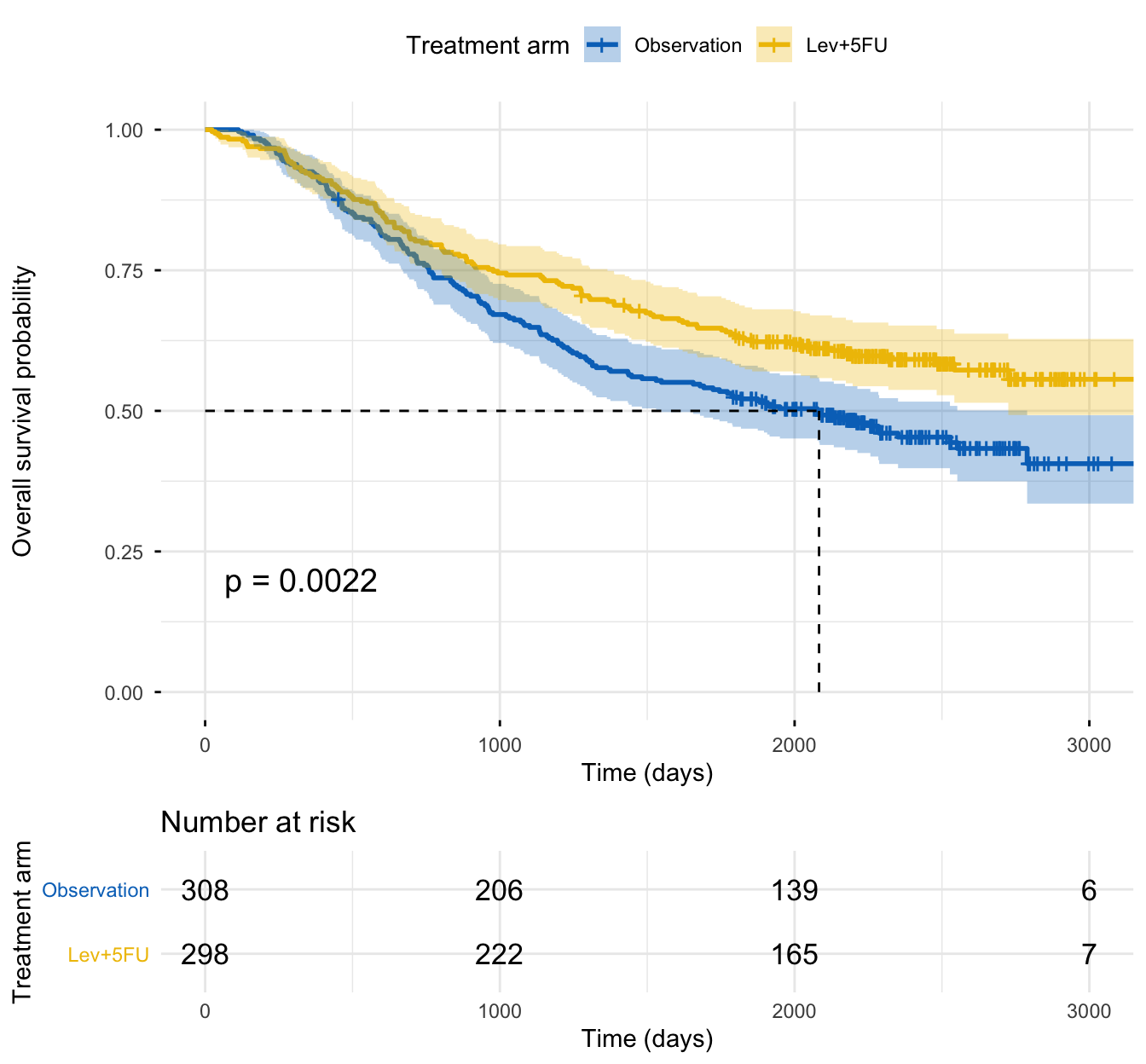
There are 606 subjects (308 Observation, 298 Lev+5FU) and 287 deaths; the rest are censored — alive at last follow-up.
The censoring flip: event = 1 - CNSR (read this twice)
This is the signature gotcha of regulatory survival analysis. R’s response object is Surv(time, event), where event = 1 marks the event and 0 marks censoring. CDISC’s CNSR is the opposite: 1 marks censored and 0 marks the event.
Pass CNSRstraight intoSurv() and you tell R that every censored subject had the event and every event was censored. The Kaplan-Meier curve and median survival become nonsense, and the hazard ratio is silently distorted — it does not cleanly flip to its reciprocal (the event times stay attached to the wrong subjects), it just drifts to a wrong, usually non-significant value. Worst of all it still runs with no error, so the only defense is to do the conversion every time and sanity-check the event count.
library(survival)os <-subset(colon, etype ==2& rx %in%c("Obs", "Lev+5FU"))os$rx <-droplevels(os$rx)adtte <-data.frame(AVAL = os$time, CNSR =1- os$status,TRT01P =factor(os$rx, levels =c("Obs", "Lev+5FU"),labels =c("Observation", "Lev+5FU")),STRAT =factor(ifelse(os$differ ==3, "Poor", "Well/Moderate")))adtte <- adtte[!is.na(adtte$STRAT), ]# Build the R event indicator from the CDISC censoring flagadtte$event <-1- adtte$CNSR# The Surv() response — note the '+' marks CENSORED subjects (CNSR == 1)head(Surv(adtte$AVAL, adtte$event), 10)
The + after a time (e.g. 1767+) marks a censored subject — exactly the rows where CNSR == 1. Sanity check passed: the Surv() object treats deaths as events and censored subjects as censored, the way it should.
The submission analysis set
With Surv(AVAL, event) built correctly, the rest is the standard time-to-event toolkit — but run with the endpoints and stratification the protocol pre-specified, not chosen post hoc.
Kaplan-Meier estimate and median OS with 95% CI
survfit() gives the median overall survival and its 95% confidence interval per arm — two of the headline numbers in any survival CSR:
Call: survfit(formula = Surv(AVAL, event) ~ TRT01P, data = adtte)

                     n events median 0.95LCL 0.95UCL
TRT01P=Observation 308    165   2083    1548    2789
TRT01P=Lev+5FU     298    122     NA    2725      NA
Read the headline numbers:
Observation: median OS = 2083 days (95% CI 1548–2789).
Lev+5FU: median = NA (“not reached”) — fewer than half the treated subjects died within follow-up, so the survival curve never drops to 0.5. The lower confidence bound (2725 days) tells you the median is at least that long. A “not reached” median is a good sign here, not missing data — report the lower CI bound and a fixed-time survival probability instead.
The signature regulatory figure — a Kaplan-Meier plot
The Kaplan-Meier curve with a number-at-risk table, confidence bands, median lines, and the log-rank p-value is the standard survival figure in a submission. Draw it with survminer’s ggsurvplot():
The Lev+5FU curve sits above the Observation curve at every time point — a consistent survival advantage for the active arm, with the curves clearly separated and not crossing.
The stratified log-rank test
Protocols routinely pre-specify stratification factors (here, tumour differentiation) so the treatment comparison is made within prognostic strata, removing their confounding. The stratified log-rank test does exactly that — add strata() to the formula:
Call:
survdiff(formula = Surv(AVAL, event) ~ TRT01P + strata(STRAT),
    data = adtte)

                     N Observed Expected (O-E)^2/E (O-E)^2/V
TRT01P=Observation 308      165      140      4.65      9.07
TRT01P=Lev+5FU     298      122      147      4.40      9.07

 Chisq= 9.1  on 1 degrees of freedom, p= 0.003
χ² = 9.1 on 1 df, p = 0.003 — after stratifying by tumour differentiation, the survival difference between arms is statistically significant. (The unstratified test gives a near-identical p = 0.002 here; they diverge when the strata are strongly prognostic and unevenly distributed across arms — pre-specify the stratified version when the protocol does.)
The primary estimate — the Cox hazard ratio
The log-rank test answers “do the arms differ?”; the regulatory submission also needs an effect size with a confidence interval — the hazard ratio, the primary estimand for a time-to-event endpoint. Fit a stratified Cox model so the HR matches the stratified log-rank logic:
Call:
coxph(formula = Surv(AVAL, event) ~ TRT01P + strata(STRAT), data = adtte)

  n= 606, number of events= 287

                 coef exp(coef) se(coef)      z Pr(>|z|)
TRT01PLev+5FU -0.3581    0.6990   0.1196 -2.995  0.00274 **
---
Signif. codes:  0 '***' 0.001 '**' 0.01 '*' 0.05 '.' 0.1 ' ' 1

              exp(coef) exp(-coef) lower .95 upper .95
TRT01PLev+5FU     0.699      1.431    0.5529    0.8836

Concordance= 0.544  (se = 0.016 )
Likelihood ratio test= 9.08  on 1 df,   p=0.003
Wald test            = 8.97  on 1 df,   p=0.003
Score (logrank) test = 9.07  on 1 df,   p=0.003
Interpret the full output in plain language:
exp(coef) = 0.70 — the hazard ratio for Lev+5FU vs Observation. Treatment multiplies the hazard of death by 0.70, i.e. a 30% lower hazard ((1 − 0.70) × 100). Observation is the reference arm, so the HR reads “treated vs control” — the direction the protocol intends.
95% CI = 0.55 to 0.88. Because the interval lies entirely below 1, the benefit is statistically convincing — there is no plausible value at which treatment is harmful or null.
z = −3.0, Pr(>|z|) = 0.003 — the Wald test of the coefficient against 0: significant.
Global tests (likelihood-ratio, Wald, score/log-rank) all give p = 0.003 — the model rejects “no treatment effect”. The concordance (0.54) is modest, expected for a single binary predictor.
A negative coef (−0.36) with an HR below 1 is the correct, protective direction. Had we passed CNSR straight into Surv(), the model would still have run — but on the wrong subjects: the HR drifts to a distorted, non-significant value (≈0.9 here, not the true 0.70) and the Kaplan-Meier median is badly wrong. It does not cleanly invert to 1/0.70; the danger is precisely that nothing complains.
Check the proportional-hazards assumption
A single hazard ratio is only meaningful if the treatment effect is constant over time — the proportional-hazards assumption. Pre-specified or not, a submission checks it with cox.zph() (Schoenfeld residuals):
       chisq df    p
TRT01P 0.912  1 0.34
GLOBAL 0.912  1 0.34
χ² = 0.91, p = 0.34 — well above 0.05, so there is no evidence the treatment hazard ratio changes over time. The single HR is a valid summary of the effect. (If this test were significant, the constant HR would mislead — see testing the PH assumption for the diagnostic plots and the fixes, and RMST for an estimand that doesn’t assume proportional hazards.)
The CSR-style summary table — gtsummary
A clinical study report doesn’t print raw R output; it presents clean tables. gtsummary turns the same fitted objects into submission-style tables with no manual formatting. First, the median OS and a fixed-time survival probability per arm:
At 5 years, 52% of the Observation arm versus 63% of the Lev+5FU arm are still alive — the survival advantage, now as a fixed-time estimate (useful precisely because the treated median was “not reached”).
Then the primary estimand — the Cox hazard ratio — as a tbl_regression:
Abbreviations: CI = Confidence Interval, HR = Hazard Ratio
exponentiate = TRUE reports hazard ratios (not log-hazards), with the 95% CI and p-value — the exact row that goes into the efficacy table of the CSR: HR 0.70 (95% CI 0.55, 0.88), p = 0.003, Observation as the reference.
The regulatory framing (ICH E9, kept practical)
The statistics above are only “submission-grade” if a few principles were settled before the analysis. You don’t need a compliance manual — you need to know what was pre-specified and to honour it.
NoteWhat a regulatory submission expects of a time-to-event analysis
A defined estimand (ICH E9(R1)). State precisely what you are estimating: the population (the Full Analysis Set / ITT), the endpoint (PARAMCD = OS, time from randomization to death from any cause), the treatment condition (TRT01P), the intercurrent-event strategy, and the summary measure (here, the hazard ratio). The HR is reported for that estimand, not as a generic association.
Pre-specification. The endpoint, the analysis population, the censoring rules, the test (stratified log-rank), the model (stratified Cox), and any stratification factors are fixed in the SAP before database lock and unblinding — not chosen after seeing the data.
Censoring rules, documented.CNSR, EVNTDESC, and CNSDTDESC make every subject’s status auditable: was this an event or a censoring, and on what date and why? Informative or inconsistent censoring biases the estimate, so the rules are written down and followed.
Stratification factors named in the protocol enter the stratified log-rank and Cox (above), so the treatment effect is estimated within prognostic strata.
Traceability. Every number traces from SDTM → ADaM (ADTTE) → the analysis output, reproducibly.
The point of ADTTE is that the data carries this contract: the structure, the variable names, and the flags are standardized precisely so a reviewer at the FDA or EMA can re-run your analysis and get your numbers.
Report
Overall survival was analyzed on the Full Analysis Set from the ADTTE dataset (PARAMCD = OS; n = 606, 287 deaths), comparing Lev+5FU with observation. Median overall survival was 2083 days (95% CI 1548–2789) in the observation arm and was not reached in the Lev+5FU arm; 5-year survival was 52% versus 63%. A stratified Cox model (stratified by tumour differentiation, the pre-specified factor) gave a hazard ratio of 0.70 (95% CI 0.55–0.88) in favour of Lev+5FU (stratified log-rank p = 0.003); the proportional-hazards assumption was satisfied (p = 0.34).
NoteWhen you need this audited and validated — Arkon
Everything on this page is the statistics of a submission-grade analysis. Turning it into an actual submission deliverable adds another layer: a validated, double-programmed analysis against the SAP, full SDTM→ADaM→TLF traceability, version-controlled and reproducible end to end, with a documented audit trail a regulator can follow. That production discipline — reproducible, validated, agent-assisted clinical analysis pipelines — is exactly what Arkon is built for. Use this lesson to do the analysis; reach for Arkon when it has to be audited and validated for a real filing.
Common issues
You passed CNSR straight into Surv(). This is the cardinal ADTTE error. Surv(AVAL, CNSR) tells R that censored subjects had the event and vice versa — the curves invert and the hazard ratio flips (protective ↔︎ harmful), usually with no error message. Always build event = 1 - CNSR first, and sanity-check the event count against sum(CNSR == 0).
You analyzed more than one parameter at once. ADTTE holds one row per subject per PARAMCD. If a subject has both OS and PFS records, an un-filtered survfit() silently pools two endpoints. Always subset(adtte, PARAMCD == "OS") (or your parameter) before building Surv().
You used the wrong time origin.AVAL is time from the protocol-defined origin — usually randomization, sometimes first dose or diagnosis. Don’t re-derive it from raw dates and don’t mix origins across subjects; the origin is fixed in the SAP and already baked into AVAL. Re-deriving time is a traceability break a reviewer will flag.
Frequently asked questions
NoteWhat is a CDISC ADTTE dataset?
ADTTE is the CDISC ADaM (Analysis Data Model) standard for time-to-event analysis in clinical trials. It holds one record per subject per analysis parameter (PARAMCD such as OS or PFS), with the analysis time in AVAL, the units in AVALU, and a censoring flag in CNSR. It is the analysis-ready, traceable dataset that survival analyses for regulatory submissions are run on.
NoteWhy is CNSR=1 censored when R’s status uses 1 for the event?
They are simply opposite conventions. CDISC’s CNSR flags the censoring: CNSR = 1 means censored, CNSR = 0 means the event occurred. R’s Surv(time, event) flags the event: event = 1 means the event, 0 means censored. To go from CDISC to R, build event = 1 - CNSR. Pass CNSR straight into Surv() and every result is silently corrupted — a serious error that throws no warning.
NoteHow do I build a Surv() object from an ADTTE dataset in R?
Filter to one parameter, convert the censoring flag, then call Surv(): adtte_os <- subset(adtte, PARAMCD == "OS"); adtte_os$event <- 1 - adtte_os$CNSR; Surv(adtte_os$AVAL, adtte_os$event). The + after a time marks a censored subject (the rows where CNSR == 1). This Surv() object is then the left-hand side of survfit(), survdiff(), and coxph().
NoteWhat is the primary estimand in a time-to-event analysis?
Under ICH E9(R1), the estimand specifies what you are estimating: the population (typically the Full Analysis Set / ITT), the endpoint (e.g. overall survival from randomization to death from any cause), the treatment condition, the intercurrent-event strategy, and the summary measure — for survival, usually the hazard ratio from a Cox model, with the (stratified) log-rank test as the corresponding hypothesis test. The HR is reported for that estimand, defined before the analysis.
NoteWhat is the difference between a stratified and an unstratified log-rank test?
The unstratified log-rank compares survival between arms across the whole sample. The stratified version compares them within pre-specified prognostic strata (e.g. tumour differentiation, region) and combines the within-stratum comparisons — removing those factors’ confounding. Use the stratified test (and a matching stratified Cox) when the protocol pre-specifies stratification factors. Add strata() to the formula: survdiff(Surv(AVAL, event) ~ TRT01P + strata(STRAT), data = adtte).
Test your understanding
ImportantPractice
Map it. You are handed an ADTTE dataset with columns AVAL, CNSR, and TRT01P. Write the R that builds the correct Surv() object and a Kaplan-Meier fit by arm. What single line is the one you must not get wrong, and why?
Interpret. A stratified Cox model on an ADTTE OS endpoint reports HR = 1.35 (95% CI 1.08–1.69, p = 0.009) for the experimental arm versus control. In plain words: is the experimental treatment helping or hurting, and is the result convincing? What would you check first about how Surv() was built?
TipHint
For (1): the response is Surv(AVAL, event) — and event is notCNSR. For (2): an HR above 1 means a higher hazard; a CI entirely above 1 is significant. If the direction looks surprising, suspect the CNSR flip.
TipSolution
library(survival)# 1. The correct mapping — the load-bearing line is `event = 1 - CNSR`adtte$event <-1- adtte$CNSR # CDISC CNSR -> R event indicatorfit <-survfit(Surv(AVAL, event) ~ TRT01P, data = adtte)print(fit)
The line you must not get wrong is event = 1 - CNSR. Because CDISC codes CNSR = 1 as censored (the opposite of R’s event = 1), passing CNSR directly into Surv() corrupts every result — the curves and the median become nonsense and the hazard ratio is silently wrong — usually with no error.
For question 2: HR = 1.35 means a 35% higher hazard of the event in the experimental arm — the treatment looks harmful, not helpful. It is statistically convincing: the 95% CI (1.08–1.69) lies entirely above 1 and p = 0.009. But before reporting harm, check how Surv() was built — a direction this surprising is exactly what a CNSR-not-flipped error produces. Confirm event = 1 - CNSR and that the event count matches sum(CNSR == 0), then refit — don’t assume the corrected HR is simply 1/1.35; with event and censoring swapped, the right value only appears once you rebuild Surv() correctly.
TipQuick check
In a CDISC ADTTE dataset, a subject has AVAL = 1767 and CNSR = 1. Did this subject experience the event?
NoteShow answer
No — this subject was censored. CDISC codes CNSR = 1 as censored: the subject was event-free (e.g. still alive) at 1767 days and then left observation. In R you would set event = 1 - CNSR = 0, and the Surv() object prints the time with a + (1767+) to mark censoring. Only CNSR = 0 is an event.
Conclusion
You can now take a CDISC ADTTE time-to-event endpoint through a submission-style analysis in R: map AVAL, CNSR, and TRT01P to a Surv() object — building event = 1 - CNSR so the censoring convention is right — then run the analysis set the protocol pre-specifies: a Kaplan-Meier curve with risk table, median OS with 95% CI, the stratified log-rank test, the primary Cox hazard ratio with its CI, a proportional-hazards check, and a CSR-style gtsummary table. On the CDISC-shaped adjuvant colon-cancer trial, Lev+5FU cut the hazard of death by ~30% (HR = 0.70, 95% CI 0.55–0.88, p = 0.003), with proportional hazards holding. The statistics are the same survival toolkit you already know; what makes them regulatory is the data contract, the censoring flip, and the estimand thinking around them.
Ask Prova“map my CDISC ADTTE dataset to a Surv() object — remember CNSR=1 is censored — then give me the Kaplan-Meier median with 95% CI, the stratified log-rank test, and the Cox hazard ratio as a gtsummary table” — it answers with survival + survminer + gtsummary code you can run on your own data. The runtime is the judge.Ask Prova →
Note
Every result on this page was produced by the code shown, run at build time against a pinned R environment — copy any block and run it to reproduce them.