Weighted Log-Rank Tests in R: Fleming-Harrington for Non-Proportional Hazards

When survival curves cross or the treatment effect is delayed, the standard log-rank test loses power — weight the early or late events with survdiff(rho=) and survMisc::comp()

Run weighted log-rank tests in R when proportional hazards fail. Use survdiff(rho = 1) for the early-weighted Peto-Peto test and survMisc::comp() for the Fleming-Harrington FH(p, q) family, compare the p-values against the standard log-rank test on the NCCTG lung data, and learn which weight to prespecify for delayed, early, or crossing effects — without fishing.

TipKey takeaways

• The standard log-rank test weights every event time equally and is most powerful under proportional hazards. When the treatment effect is delayed, early then fading, or the curves cross, that equal weighting dilutes the signal — a weighted log-rank test is more powerful.
• A weighted test multiplies each time point’s observed-minus-expected contribution by a weight. Push the weight toward early event times or late ones, depending on where the difference lives.
• The quick route is base survdiff(..., rho = 1) — the Peto-Peto test, which emphasizes early differences; rho = 0 is the standard test. The full family is Fleming-Harrington FH(p, q) via survMisc::comp() — FH(1, 0) early, FH(0, 1) late.
• On the lung data the sex difference is concentrated early: standard χ² = 10.3, p = 0.0013; early-weighted FH(1, 0) χ² = 12.7, p = 0.0004 (stronger); late-weighted FH(0, 1) χ² = 3.5, p = 0.063 (nearly misses it).
• Prespecify the weight from the biology — never fish. Trying every weight and reporting the smallest p inflates the type-I error. Choose one test before you look at the data; the rest are sensitivity analyses. Always read the proportional-hazards check first.

Introduction

The log-rank test is the default for comparing survival between groups, and for good reason — but it has one blind spot. It gives equal weight to every event time, which makes it the most powerful test only when the hazard ratio is roughly constant over follow-up (proportional hazards). Modern trials routinely break that assumption:

• Delayed effect — immunotherapy and cancer vaccines often show no separation for months, then a growing benefit. The early non-difference drags the standard test toward “no effect.”
• Early effect that fades — a cytotoxic drug separates the curves fast, then resistance erodes the gap.
• Crossing curves — an aggressive therapy with early toxicity but a long-term benefit: early and late differences point in opposite directions and cancel in the standard test.

In all three cases the standard log-rank test loses power and can miss a real difference. A weighted log-rank test fixes this by emphasizing the part of follow-up where the difference actually lives. This lesson runs them in R — the quick Peto-Peto test with base survdiff(..., rho = ), then the full Fleming-Harrington FH(p, q) family with survMisc — on the NCCTG lung-cancer data, comparing every result against the standard test.

ImportantThis is the non-PH remedy — check first

A weighted log-rank test is the answer to a specific problem: non-proportional hazards. Before reaching for it, confirm the problem exists — inspect the Kaplan-Meier curves and run the formal check in Testing the proportional hazards assumption (cox.zph()). If hazards are proportional, the standard log-rank test is the most powerful choice and a weighted test only costs you power.

The weight idea: early vs late emphasis

The log-rank statistic accumulates, across every event time \(t_i\), the gap between the observed events in a group and the expected events under H₀. A weighted test multiplies each gap by a weight \(w(t_i)\) before summing:

• All weights equal (\(w = 1\)) → the standard log-rank test. Every event time counts the same.
• Weights large early, small late → an early-emphasis test. A difference in the first months dominates; a late difference barely registers.
• Weights small early, large late → a late-emphasis test. The right choice for a delayed effect (immunotherapy), where the curves only separate after the early period.

The Fleming-Harrington family parametrises the weight with two numbers, p and q, applied to the pooled Kaplan-Meier survival estimate \(\hat S(t)\):

\[ w(t_i) = \hat S(t_i)^{\,p} \cdot \left[1 - \hat S(t_i)\right]^{\,q} \]

Early in follow-up \(\hat S(t)\) is near 1, so \(\hat S(t)^p\) is large and \([1-\hat S(t)]^q\) is small; late in follow-up the reverse holds. That gives a clean dial:

• FH(0, 0) → \(w = 1\): the standard log-rank test.
• FH(1, 0) → \(w = \hat S(t)\): early emphasis (weight high while survival is high).
• FH(0, 1) → \(w = 1 - \hat S(t)\): late emphasis (weight grows as patients die — for delayed effects).
• FH(1, 1) → maximum weight in the middle of follow-up.

NoteA naming trap worth knowing

The base survdiff() function takes a single parameter, rho, which is not the Fleming-Harrington p. survdiff(rho = 0) is the standard test; survdiff(rho = 1) is the Peto-Peto test, which weights by \(\hat S(t)\) — early emphasis (equivalent to Fleming-Harrington FH(1, 0)). For the full two-parameter family — including late emphasis — use survMisc::comp(), which takes p and q directly.

The data: the NCCTG lung-cancer study

We use lung, the North Central Cancer Treatment Group dataset from the survival package: survival in 228 patients with advanced lung cancer. With survival attached, lung is available directly — no data() call needed. We compare survival by sex (1 = male, 2 = female):

library(survival)

head(lung[, c("time", "status", "sex")])

  time status sex
1  306      2   1
2  455      2   1
3 1010      1   1
4  210      2   1
5  883      2   1
6 1022      1   1

• time — survival time in days.
• status — 1 = censored, 2 = dead (the event).
• sex — 1 = male, 2 = female (the grouping variable).

Look at the curves before testing anything. The hero plot below marks the early stretch of follow-up — the period an early-weighted test emphasizes:

library(survival)
library(survminer)

fit <- survfit(Surv(time, status) ~ sex, data = lung)

ggsurvplot(
  fit,
  data = lung,
  conf.int = TRUE,
  palette = "jco",                       # colourblind-safe journal palette
  legend.labs = c("Male", "Female"),
  legend.title = "Sex",
  xlab = "Time (days)",
  ylab = "Survival probability",
  ggtheme = theme_minimal()
)$plot +
  ggplot2::annotate(
    "rect", xmin = 0, xmax = 300, ymin = 0, ymax = 1,
    alpha = 0.08, fill = "#3a86d4"
  ) +
  ggplot2::annotate(
    "text", x = 150, y = 0.05, label = "early emphasis",
    size = 3, colour = "#3a86d4"
  )

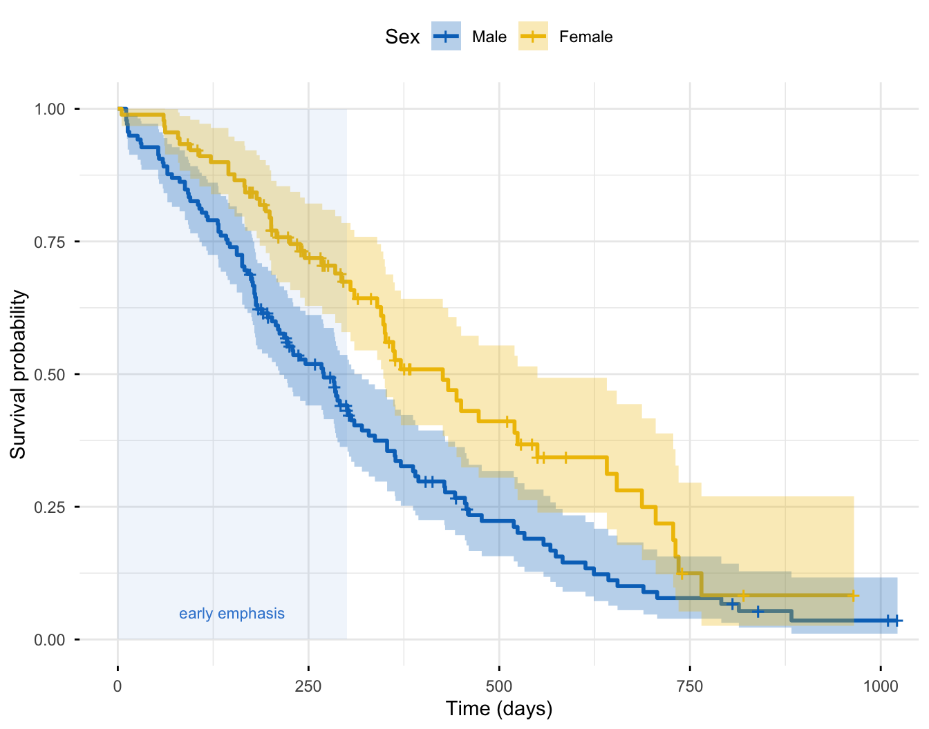
The curves separate early — the female curve pulls above the male curve within the first few hundred days — and the gap is widest while most patients are still at risk. That shape predicts what we are about to see: an early-weighted test will be the most powerful here, and a late-weighted one will be the weakest.

The quick route: survdiff(rho = ) (Peto-Peto)

Base survdiff() gives you a one-parameter weighted test for free. rho = 0 is the standard log-rank test; rho = 1 is the Peto-Peto test, which weights by \(\hat S(t)\) — early emphasis. Run both and compare:

library(survival)

# rho = 0: the standard log-rank test (equal weights)
survdiff(Surv(time, status) ~ sex, data = lung, rho = 0)

Call:
survdiff(formula = Surv(time, status) ~ sex, data = lung, rho = 0)

        N Observed Expected (O-E)^2/E (O-E)^2/V
sex=1 138      112     91.6      4.55      10.3
sex=2  90       53     73.4      5.68      10.3

 Chisq= 10.3  on 1 degrees of freedom, p= 0.001 

library(survival)

# rho = 1: the Peto-Peto test — early-weighted
survdiff(Surv(time, status) ~ sex, data = lung, rho = 1)

Call:
survdiff(formula = Surv(time, status) ~ sex, data = lung, rho = 1)

        N Observed Expected (O-E)^2/E (O-E)^2/V
sex=1 138     70.4     55.6      3.95      12.7
sex=2  90     28.7     43.5      5.04      12.7

 Chisq= 12.7  on 1 degrees of freedom, p= 4e-04 

Read the two side by side:

• Standard (rho = 0): χ² = 10.3 on 1 df, p = 0.0013. Survival differs significantly between the sexes — the result you would report under proportional hazards.
• Peto-Peto (rho = 1): χ² = 12.7 on 1 df, p = 0.0004. The early-weighted test is more significant (a larger χ², a smaller p). That is the signature of an early difference: putting more weight on the first event times — where the curves are furthest apart and the most patients are at risk — sharpens the signal.

Notice the Observed and Expected counts in the rho = 1 table are fractional and smaller than in the standard table: they are weighted event counts, not raw deaths. That is expected — only the χ² and p-value are comparable across the two tests.

The full family: Fleming-Harrington FH(p, q) with survMisc

survdiff() only dials early emphasis. For the complete two-parameter family — including late emphasis for delayed effects — use survMisc::comp(). It takes a ten object (built from a survfit() fit) and vectors of p and q values, then runs every Fleming-Harrington weight at once:

library(survival)
library(survMisc)

fit <- survfit(Surv(time, status) ~ sex, data = lung)

# FH(1,0) early-weighted and FH(0,1) late-weighted, alongside the standard FH(0,0)
fh <- comp(ten(fit), p = c(1, 0), q = c(0, 1))

                     Q         Var       Z pNorm
1             -20.4183     40.4280 -3.2113     6
n           -3148.0000 795286.3234 -3.5300     4
sqrtN        -248.2336   4952.6740 -3.5273     5
S1            -14.6872     16.9922 -3.5630     3
S2            -14.5848     16.7542 -3.5632     2
FH_p=1_q=0    -14.8065     17.2608 -3.5639     1
FH_p=0_q=1     -5.6118      9.1175 -1.8585     7
              maxAbsZ        Var      Q pSupBr
1          2.2095e+01 4.0428e+01 3.4750      6
n          3.1750e+03 7.9529e+05 3.5603      5
sqrtN      2.5507e+02 4.9527e+03 3.6244      1
S1         1.4917e+01 1.6992e+01 3.6188      3
S2         1.4802e+01 1.6754e+01 3.6163      4
FH_p=1_q=0 1.5039e+01 1.7261e+01 3.6198      2
FH_p=0_q=1 7.0563e+00 9.1175e+00 2.3369      7

comp() prints a compact table of several weight families; the pNorm column on the printout is a rank (1 = most significant), not the p-value — the actual statistics live in the fitted object. Pull the three we care about into a clean summary:

library(survival)
library(survMisc)

fit <- survfit(Surv(time, status) ~ sex, data = lung)

t1 <- ten(fit)
invisible(comp(t1, p = c(1, 0), q = c(0, 1)))   # run the tests, suppress the table

                     Q         Var       Z pNorm
1             -20.4183     40.4280 -3.2113     6
n           -3148.0000 795286.3234 -3.5300     4
sqrtN        -248.2336   4952.6740 -3.5273     5
S1            -14.6872     16.9922 -3.5630     3
S2            -14.5848     16.7542 -3.5632     2
FH_p=1_q=0    -14.8065     17.2608 -3.5639     1
FH_p=0_q=1     -5.6118      9.1175 -1.8585     7
              maxAbsZ        Var      Q pSupBr
1          2.2095e+01 4.0428e+01 3.4750      6
n          3.1750e+03 7.9529e+05 3.5603      5
sqrtN      2.5507e+02 4.9527e+03 3.6244      1
S1         1.4917e+01 1.6992e+01 3.6188      3
S2         1.4802e+01 1.6754e+01 3.6163      4
FH_p=1_q=0 1.5039e+01 1.7261e+01 3.6198      2
FH_p=0_q=1 7.0563e+00 9.1175e+00 2.3369      7

lrt <- attr(t1, "lrt")                          # the log-rank-test results table
idx <- match(c("1", "FH_p=1_q=0", "FH_p=0_q=1"), as.character(lrt$W))

data.frame(
  Test    = c("FH(0,0) standard", "FH(1,0) early emphasis", "FH(0,1) late emphasis"),
  ChiSq   = round(lrt$chiSq[idx], 2),
  p_value = signif(lrt$pChisq[idx], 3)
)

                    Test ChiSq  p_value
1       FH(0,0) standard 10.31 0.001320
2 FH(1,0) early emphasis 12.70 0.000365
3  FH(0,1) late emphasis  3.45 0.063100

Read the family in plain language:

• FH(0, 0) standard — χ² = 10.3, p = 0.0013. The equal-weight baseline (it matches survdiff(rho = 0)).
• FH(1, 0) early emphasis — χ² = 12.7, p = 0.0004. The most powerful test here, matching the Peto-Peto result — because the sex difference is an early one.
• FH(0, 1) late emphasis — χ² = 3.5, p = 0.063. The weakest test: it weights the late event times, where the curves have nearly converged and few patients remain — so it almost misses a difference that is genuinely there.

That last row is the whole lesson in one number. A late-emphasis test applied to an early effect (or vice versa) can flip a clearly significant result into a non-significant one. The weight must match where the difference is — and you must decide which weight before you see the data.

When to use which weight

TipMatch the weight to the expected effect — prespecified

• Proportional hazards (curves stay roughly parallel, don’t cross) → the standard log-rank test, FH(0, 0) / survdiff(rho = 0). A weighted test only costs power here.
• Delayed effect (no early separation, then growing benefit — immunotherapy, vaccines) → late emphasis, FH(0, 1) via comp(..., p = 0, q = 1).
• Early effect that fades (fast separation, then convergence) → early emphasis, FH(1, 0) / survdiff(rho = 1) (Peto-Peto).
• Crossing curves → a weighted test in either direction beats the standard test (which cancels the opposing differences), but state the clinical question first; consider restricted mean survival time as a complementary summary that does not depend on a weight choice.

ImportantDon’t fish across weights — prespecify

Every weight you try is another test. Running FH(0,0), FH(1,0), FH(0,1), FH(1,1), … and reporting the smallest p-value inflates the type-I error rate far above 5% — you will “find” significant effects in pure noise. The fix is procedural, not statistical:

• Choose one weight before unblinding, justified by the biology (the mechanism’s expected timing) or by prior data — and report that test as primary.
• Treat the other weights as prespecified sensitivity analyses, not competing primary results.
• If you genuinely cannot predict the pattern, a combination test (e.g. MaxCombo, which takes the maximum over a small prespecified set of weights with a proper multiplicity adjustment) controls the error — that is a deliberate design choice, not post-hoc weight-shopping.

The one thing you must never do is scan every weight and report the best.

Report

Survival was compared between male and female patients on the NCCTG lung-cancer data (n = 228, 165 deaths). Because the Kaplan-Meier curves separated early in follow-up, a prespecified early-weighted Fleming-Harrington test, FH(1, 0) (Peto-Peto, survdiff rho = 1), was the primary comparison: survival differed significantly between the sexes (χ²(1) = 12.7, p = 0.0004). The standard log-rank test agreed (χ²(1) = 10.3, p = 0.0013); a late-emphasis test FH(0, 1) was weaker (χ²(1) = 3.5, p = 0.063), consistent with an early difference. Females survived longer (median 426 vs 270 days).

NoteThe math behind the weighted log-rank statistic (optional)

At each distinct event time \(t_i\), with \(d_i\) events among \(n_i\) patients at risk, let \(O_{1i}\) and \(E_{1i}\) be the observed and expected events in group 1, and \(V_i\) the variance — exactly the log-rank ingredients. The weighted statistic attaches a weight \(w_i\) to each term:

\[ Z_w = \frac{\sum_i w_i \,(O_{1i} - E_{1i})}{\sqrt{\sum_i w_i^2 \, V_i}} \]

and \(Z_w^2\) follows a chi-square distribution with 1 degree of freedom. Setting all \(w_i = 1\) recovers the standard log-rank test. The Fleming-Harrington weight is \(w_i = \hat S(t_i)^{\,p}\,[1 - \hat S(t_i)]^{\,q}\), where \(\hat S\) is the pooled Kaplan-Meier estimate just before \(t_i\): with \(p > 0\) the weight is large while survival is high (early), and with \(q > 0\) it grows as survival falls (late). Because the weight is fixed by \((p, q)\) before seeing group membership, a prespecified choice is a valid test; choosing \((p, q)\) to minimise the observed \(p\)-value is not.

Try it live

Run the weighted tests yourself — change the grouping variable, or dial the FH(p, q) weights. The sandbox boots on first Run.

🟢 With an AI agent

Ask Prova “my survival curves separate late — pick and run a weighted log-rank test in R that emphasizes late differences, compare it to the standard log-rank test, and tell me which to prespecify” — it answers with survival + survMisc code you can run on your own data. The runtime is the judge. Ask Prova →

Common issues

You ran every weight and reported the smallest p-value. This inflates the type-I error rate well above 5% — the single most common misuse of weighted tests. Prespecify one weight from the biology before unblinding and treat the rest as sensitivity analyses; if the pattern is genuinely unknown, use a multiplicity-controlled combination test (MaxCombo), not weight-shopping.

Your curves cross and even the weighted test looks weak. A single weight emphasizes one direction of difference; when curves cross, early and late differences oppose each other and any single-weight test can still struggle. State the clinical question (is early or late survival what matters?) and consider restricted mean survival time as a weight-free complementary summary.

The Observed/Expected counts in survdiff(rho = 1) look wrong (fractional, too small). They are weighted event counts, not raw deaths — only the χ² statistic and the p-value are comparable to the standard test. Don’t try to reconcile the weighted counts with the actual number of deaths.

Frequently asked questions

NoteWhen should I use a weighted log-rank test instead of the standard one?

Use a weighted log-rank test when the proportional-hazards assumption fails — the survival curves cross, the treatment effect is delayed (immunotherapy), or it is early and then fades. In those cases the standard log-rank test gives equal weight to every time point and loses power. If hazards are proportional (curves stay roughly parallel and don’t cross), the standard log-rank test is the most powerful choice and a weighted test only costs you power — so check the curves and run cox.zph() first.

NoteWhat is the difference between rho in survdiff() and the Fleming-Harrington p and q?

survdiff() exposes a single parameter, rho. rho = 0 is the standard log-rank test; rho = 1 is the Peto-Peto test, which weights by the survival estimate \(\hat S(t)\) — early emphasis (equivalent to Fleming-Harrington FH(1, 0)). The Fleming-Harrington family has two parameters, p and q, with weight \(\hat S(t)^p [1 - \hat S(t)]^q\) — p drives early emphasis, q drives late emphasis. For late emphasis (a delayed effect) you need survMisc::comp(..., p = 0, q = 1); survdiff() alone cannot do it.

NoteWhich weight do I use for an immunotherapy / delayed treatment effect?

A late-emphasis weight — Fleming-Harrington FH(0, 1) (comp(ten(fit), p = 0, q = 1)). Delayed effects show no early separation, then a growing benefit, so the difference lives in the later event times; weighting them up recovers the power the standard test loses. Prespecify this weight from the mechanism before unblinding, and report the standard log-rank test as a sensitivity analysis.

NoteCan I try several weights and report the most significant one?

No. Each weight is a separate test, so scanning many and reporting the smallest p-value inflates the type-I error rate — you will find “significant” effects in noise. Prespecify one weight (from the biology or prior data) as primary and treat the others as sensitivity analyses. If you genuinely cannot predict the effect’s timing, use a MaxCombo combination test, which takes the maximum over a small prespecified set of weights with a proper multiplicity adjustment.

NoteHow is a weighted log-rank test related to the Cox model?

The standard log-rank test corresponds to a Cox model with a constant hazard ratio. When hazards are non-proportional, neither a single hazard ratio nor the standard log-rank test summarises the effect well. A weighted log-rank test gives a more powerful p-value for “do the curves differ?”, but still no effect size. To describe a time-varying effect, fit a Cox model with time-varying coefficients or report restricted mean survival time; see Testing the proportional hazards assumption for diagnosing the violation in the first place.

Test your understanding

ImportantPractice

1. Run it. In the live cell below, the curves are compared by ECOG performance score (ph.ecog). Fill the blank to run an early-weighted Peto-Peto test, and compare its p-value to the standard log-rank test. Does the early weighting strengthen or weaken the evidence?
2. Choose a weight. A phase III immunotherapy trial shows identical survival for the first 6 months, then the treatment curve pulls clearly above control. Which Fleming-Harrington weight should be the prespecified primary test, and why?

NoteHint

For an early-weighted (Peto-Peto) test, set rho = 1 — rho = 0 is the standard test. Compare the Chisq and p lines from the two survdiff() calls. For question 2, a delayed effect lives in the late event times, so you need late emphasis.

NoteSolution

survdiff(Surv(time, status) ~ ph.ecog, data = lung, rho = 1)
#> An early-weighted (Peto-Peto) test of survival across ECOG groups.
#> Compare its Chisq / p to the rho = 0 standard test: because worse
#> performance scores separate early, the early weighting strengthens
#> the evidence (a larger Chisq, a smaller p) here.

For question 2: the effect is delayed — no early difference, then a late benefit — so the difference lives in the late event times. Prespecify a late-emphasis test, Fleming-Harrington FH(0, 1) (comp(ten(fit), p = 0, q = 1)), justified by the immunotherapy mechanism. A standard log-rank test would be diluted by the early non-difference, and an early-weighted test would point exactly the wrong way.

TipQuick check

You expect a delayed treatment benefit (curves separate only after several months). You run survdiff(Surv(time, status) ~ arm, data = trial, rho = 1) as your primary test. Is that the right choice?

NoteShow answer

No. rho = 1 is the Peto-Peto / early-emphasis test — it weights the early event times, exactly where a delayed effect shows no difference, so it would lose power. For a delayed effect you need a late-emphasis test, Fleming-Harrington FH(0, 1) via survMisc::comp(ten(fit), p = 0, q = 1). The rho direction is the opposite of what the name might suggest — rho = 1 emphasizes early, not late.

Conclusion

When proportional hazards fail — delayed effects, early-then-fading effects, crossing curves — the standard log-rank test loses power because it weights every event time equally. A weighted log-rank test restores that power by emphasizing the part of follow-up where the difference lives: survdiff(..., rho = 1) for a quick early-weighted (Peto-Peto) test, and survMisc::comp() for the full Fleming-Harrington FH(p, q) family — FH(1, 0) early, FH(0, 1) late. On the lung data the sex difference was an early one, so the early-weighted test was strongest (χ² = 12.7, p = 0.0004) and the late-weighted test nearly missed it (p = 0.063) — a reminder that the weight must match the effect, and that you must prespecify it rather than fish across weights. Diagnose the non-proportionality first with the PH check; choose one weight from the biology; report the rest as sensitivity analyses.

Related lessons

• Log-rank test — the standard, equal-weight comparison this lesson extends; start here if hazards are proportional. · Testing the proportional hazards assumption — diagnose the non-proportionality (crossing/delayed effects) that makes a weighted test necessary; run this first. · Stratified log-rank — the other variant, for adjusting a group comparison for a confounder. · Cox proportional hazards model — quantify the difference as a hazard ratio when hazards are proportional.
• Go further: Survival Analysis — the full series. · Biostatistics — the pillar.

Was this page helpful?

Prove you can do it. Master the whole Survival Analysis in R series — track your path, build projects, and earn a certificate.

Start free →

Go Pro — unlimited Prova on your own data and a verifiable certificate that proves the skill.

from $15/mo billed yearly

Go Pro →

✓ You're Pro — keep going. The runtime is the judge.

Ready to level up?

Try this on your own data with Prova — the runtime is the judge.Open Prova →

Get new R & Python lessons by email

Practical, reproducible, no spam. Unsubscribe anytime.

Double opt-in. We never share your email.

Share this pageXLinkedInRedditHN

Note

Every result on this page was produced by the code shown, run at build time against a pinned R environment — edit any block and Run to reproduce it yourself.